Molecular Anions


Jack Simons, Chemistry Department, Henry Eyring Center for Theoretical Chemistry, University of Utah
This web-based text book offers many web links to researchers who have contributed much to the study of molecular anions. It also offers many literature references pertaining to the examples I use to illustrate the families of molecular anions discussed. It is my hope that the reader will find this text to be a useful resource for learning why the experimental and theoretical study of anions is such an exciting endeavor for so many chemists. I also hope it contains some surprises that offer even the most knowledgeable reader some new insight into the behavior of negative molecular ions. If I have been successful, I am confident that wonderful new knowledge about molecular anions will be produced by readers of this text and that new workers will be drawn to this exciting field of study.
I am still working out the bugs encountered in posting the html version on the web (e.g., the Greek and math symbols). If you want to offer input for future improvements or additions, send me an email.
I hope you enjoy browsing through this text and connecting to its many web links.
Table of Contents
- Introduction
- Chpt 1. Introduction to Molecular Anions
- Chpt 2. Anions Also Present Special Challenges to Theoretical Study
- I. Special Atomic Basis Sets Must be Used
- II. The Hartree-Fock SCF Process is Usually the Starting Point
- III. Koopmans' Theorem Gives the First Approximation to the Electron Affinity
- IV. Electron Correlation Involving the Excess Electron Usually Must be Treated
- V. Various Methods Can be Used to Treat Correlation
- VI. Computational Requirements, Strengths, and Weaknesses of Various Methods
- VII. Direct Calculation of Intensive Energy Methods
- VIII. Complete Basis Extrapolations
- IX. Why is Electron Correlation So Important for EAs?
- X. Reaction Paths
- XI. Summary
- Chpt 3. Chemically Conventional Anions
- Chpt 4. Multipole-Bound Anions
- Chpt 5. Multiply Charged Anions
- Chpt 6. Cluster Anions
- Chpt 7. Anions of Biological Molecules
- References
Introduction
Within the pages of this book, my personal perspectives are offered on the chemical study of negative molecular ions. Not much emphasis will be placed on discussing atomic anions as isolated species because it is my view that chemistry deals primarily with molecules and materials and with their reactions and properties, and I think the world of molecules begins with two or more atoms held together by chemical bonds. Therefore, I view the study of isolated atomic anions as primarily the domain of the atomic physics community although, of course, I do think it useful to discuss atoms as building blocks that form molecules. A recent review by Professor David J. Pegg from the point of view of a physicist with emphasis on atomic anions can be found at this online link.
For insight into the experimental study of negative molecular ions from a chemist's point of view beyond what is presented in this text, I refer the reader to the web sites of Professor W. C. Lineberger and Professor John I. Brauman.
 Carl Lineberger, University of Colorado
 John Brauman, Stanford University
These two scholars have done as much if not more than anyone else over the past forty years to contribute to chemists' knowledge about electron affinities and the chemical structures, reactions, and spectroscopy of molecular anions. Their groups have also pioneered many of the most useful experimental tools for studying molecular anions and have generated many scientific offspring who became major figures in this field. Of course, even they stood on the shoulders of earlier masters such as Louis Branscomb (Atomic and Molecular Processes, edited by D. R. Bates, Academic Press, New York, N.Y. (1962)), George Schulz (Rev. Mod. Phys. 45, 373, 423 (1973)), and Sir H. S. W. Massey (Negative Ions, Cambridge Univ. Press (1976), Cambridge, England).
I will make use of many examples of chemical studies carried out by Professors Brauman and Lineberger as well as results from the laboratories of many others I mention throughout this text. In so doing, I do not mean to suggest that only the groups I mention in each example have contributed to such studies; in fact, most of the groups I highlight pursue work on many if not most of the molecular anions treated in this book. For brevity, I have chosen to discuss a few examples for each of the classes of anions treated.
Many other senior scholars have contributed much to the advancement of experimental studies of molecular anions in recent decades and continue to do so. Several of them are shown below. They and many of their scientific offspring continue to expand the horizons of this field of study.

Kit Bowen, Johns Hopkins

Jim Coe, Ohio State

Dan Neumark, Berkeley

Bob Compton, Tennessee

Mark Johnson, Yale

Torkild Andersen, Aarhus

Lars Andersen, Aarhus

Paul Burrow, Nebraska

Lai-Sheng Wang, Washington State

Jack Beauchamp, Caltech

Kent Ervin, Nevada, Reno

Michael Allan, Fribourg

Veronica Bierbaum, Colorado

Barney Ellison, Colorado

Eugen Illenberger, Berlin

Léon Sanche, Sherbrooke

Ron Naaman, Weizmann

Tilmann Märk, Innsbruck

Paul Kebarle, Alberta
The University of Colorado's Joint Institute for Laboratory Astrophysics (JILA) has a very long tradition of experimental advances and studies of molecular anions. Below we see several JILA scientists whose scientific careers are linked strongly to this field of study; can you identify them?

The University of Colorado, JILA, Ion Gang in 1980.
Throughout this text, I will show many examples from labs of the people shown in the above figures of experimental data on a wide range of molecular anions.
Of course, there have been theoretical chemists who have also advanced our knowledge of molecular anions during the same timeframe. Professor R. S. Berry was among the earliest pioneers (R. S. Berry, Chem. Rev. 69, 533 (1969)) of such studies.

Steve Berry, Chicago
Several other senior chemistry scholars who have contributed much to the advancement of the theoretical study of molecular ions are shown below.

Lenz Cederbaum, Heidelberg

Alex Boldyrev, Utah State

Ken Jordan, Pittsburgh

Josef Kalcher, Gratz

Piotr Skurski, Gdansk

Maciej Gutowski, Edinburgh

Vince Ortiz, Auburn

Ludwik Adamowicz, Arizona

Howard Taylor, USC

Fritz Schaefer, Georgia

Ernest Davidson, Washington

Kwang Kim, Pohang
I will also show results from these scientists' research efforts throughout this text.
Prior to the time most of the people shown above began to contribute to molecular anion chemistry, the electron affinities of most atoms were not known and very little was known about the electron affinities of molecules and radicals. It was largely because of experimental advances in ion sources and spectroscopic probes that the determination of molecular electron affinities and the study of molecular anions began to advance rapidly in the 1960s and 1970s. Once experimental chemists began to be able to make and study negative molecular ions, it was natural for theoretical chemists to become involved in this field. However, they too faced significant challenges and had to develop new models and new computational tools to study anions as I will show later in this text.
My own history in the field dates to 1973, when our first paper (Theory of Electron Affinities of Small Molecules, J. Simons, and W. D. Smith, J. Chem. Phys., 50, 4899-4907 (1973)) dealing with the ab initio calculation of electron affinities (EAs) using what we termed the equations of motion (EOM) method was published. At about this same time, Professor Lenz Cederbaum was developing what turned out to be an equivalent method [[1]] for directly calculating ion-molecule energy differences, as were other groups [[2]]. Prior to this time, quantum chemical calculations of molecular EAs [[3]] were most commonly carried out using approximate solutions to the Schrödinger equations to obtain the total electronic energies of the neutral (Eneu) and anionic (Ean) species and subtracting these two quantities to compute the EA as
EA = Eneu – Ean.
However, because the EA is a very small fraction of the total electronic energies of the neutral or the anion, this process is fraught with danger because one must obtain each of the two total energies to very high percent accuracies to obtain the EA to a chemically useful accuracy. To illustrate, we note that EAs typically lie in the 0.01-5 eV range, but the total electronic energy of even a small molecule is usually several orders of magnitude larger. For example, the EA of the 4S3/2 state of the carbon atom is [[4]] 1.262119 ± 0.000020 eV, whereas the total electronic energy of this state of C is
–1030.080 eV (this total energy is defined relative to a C6+ nucleus and six electrons infinitely distant and not moving). Since the EA is ca. 0.1 % of the total energy of C, one needs to compute the C and C- electronic energies to accuracies of 0.01 % or better to calculate the EA to within 10%.
Moreover, because the EA is an intensive quantity but the total energy is an extensive quantity, the difficulty in evaluating EAs to within a fixed specified (e.g., ± 0.1 eV) accuracy based on subtracting total energies becomes more and more difficult
as the size and number of electrons in the molecule grows. For example, the EA of
C2 in its X ![]() ground electronic state [4] is 3.269 ± 0.006 eV near the equilibrium bond length Re but only 1.2621 eV at R →∞ (i.e., the same as the EA of a carbon atom). However, the total electronic energy
of C2 is –2060.160 eV at R →∞ and lower by ca. 3.6 eV (the dissociation energy [[5]] of C2) at Re, so again the EA is a very small fraction of the total energies. For buckyball C60, the EA is [4] 2.666 0.001 eV, but the total electronic energy is sixty times –1030.080
eV minus the atomization energy (i.e., the energy change for C60 → 60 C) of this compound. This situation becomes especially problematic when studying
extended systems such as solids, polymers, or surfaces for which the EA is an infinitesimal
fraction of the total energy. I should note that this same difficulty plagues the
theoretical evaluation of other intensive properties such as ionization potentials,
electronic excitation energies, bond energies, heats of formation, etc.
ground electronic state [4] is 3.269 ± 0.006 eV near the equilibrium bond length Re but only 1.2621 eV at R →∞ (i.e., the same as the EA of a carbon atom). However, the total electronic energy
of C2 is –2060.160 eV at R →∞ and lower by ca. 3.6 eV (the dissociation energy [[5]] of C2) at Re, so again the EA is a very small fraction of the total energies. For buckyball C60, the EA is [4] 2.666 0.001 eV, but the total electronic energy is sixty times –1030.080
eV minus the atomization energy (i.e., the energy change for C60 → 60 C) of this compound. This situation becomes especially problematic when studying
extended systems such as solids, polymers, or surfaces for which the EA is an infinitesimal
fraction of the total energy. I should note that this same difficulty plagues the
theoretical evaluation of other intensive properties such as ionization potentials,
electronic excitation energies, bond energies, heats of formation, etc.
These examples show that computing the EA of a molecule by using the total energies of its neutral and anion may not be a wise approach. How do most experiments determine molecular EAs? The most direct technique involves using a tunable light source of frequency n to photodetach an electron from a molecular anion A-. By determining the minimum photon energy hn needed to detach an electron to form the neutral molecule A, one determines the EA. This offers an example of how the EA is determined directly. Nowhere in this experiment is the extensive total energy of either the anion or the neutral measured. So, it would appear natural to seek a theoretical approach to determining EAs that follows the experimental example.
In the 1973 paper mentioned above, we did so by developing the equations of motion (EOM) method as a route to calculating the intensive EAs directly as eigenvalues of a set of working equations. In this theoretical development, one avoids (approximately) solving the Schrödinger equation for the extensive energies of the neutral and anion and then subtracting the two extensive energies to obtain the desired intensive EA. In numerous of our subsequent publications, the EOM method was refined and applied to a variety of molecular anions. In the intervening years, our group and others [[6]] have greatly extended the EOM method beyond the Møller-Plesset framework that we initially used to allow more powerful coupled-cluster, multi-configurational, and other wave function classes to be employed. Most of the subsequent developments of these theoretical tools have been cast within the language of so-called Greens function or propagators, but they could just as well have been written in our EOM language. As a result of such advances by many different groups, several direct-calculation techniques are now routinely used to compute EAs; that of Professor Vince Ortiz [6] is even contained within the widely used Gaussian suite of programs [[7]] that many chemists use routinely.
In the early studies of anions carried out in the 1970s and 80, emphasis was placed on simply determining electron affinities (EAs) rather than on probing the potential energy surfaces of chemical reactions involving anions, determining their spectrocsopic and structural properties, or attempting to design anions with novel structural or bonding characters. This was true both of the theoretical and experimental investigation of anions primarily because
- prior to 1970, even these most fundamental thermodynamic data (i.e., EAs) had not been directly (i.e., by laser photodetachment) determined for most atoms, molecules, and radicals, and
- the experimental and theoretical tools available to determine EAs were in their formative stages and needed to be tested on species whose EAs were reasonably well known from other sources.
In the subsequent thirty years, the field has broadened considerably to where the study of molecular anions is now motivated by a variety of reasons including designing new anions having specific bonding behavior or energy content and probing the influence of electrons attached to biological molecules, water clusters, interfaces, and within nanoscopic materials. Over this same period, the number of research groups focusing on anion chemistry has grown tremendously. In the 1970s, issues of J. Chem. Phys. or J. Phys. Chem. contained very few papers on anions, but now essentially any issue of either of these journals contains more than one anion paper and the number and range of such papers in increasing rapidly.
Because our knowledge of molecular anions has reached a stage in which the field has very broad interest and impact, I felt it was time to offer a source from which one could gain perspective about these species. By no means does this book intend to thoroughly review the vast body of knowledge that has been established on molecular anions' properties or to tabulate molecular EAs. Rather, it focuses on providing references to many practicing scientists and other valuable sources of information and on introducing the reader to
- the fundamental properties that make anions qualitatively different from neutrals and cations,
- introducing several classes of anions whose study has substantially expanded in recent years but which still offer promise of many more discoveries.
- illustrating the special challenges that the study of molecular anions present.
In my mind, this book is a text from which one can learn rather than a reference book where one can look up all that is known.
If one is searching for tabulated values of atomic or molecular electron affinities (EAs), the best places to search for such information are:
- For atoms, the early reviews of Hotop and Lineberger [[8]], and the more recent review by Andersen, Haugen, and Hotop [[9]] remain excellent sources.
- For molecules, there are several sources [[10], [11], [12], [13], [14]] that span many years, some of which are accessible on the web.
The primary focus of the present work is to first (Chapters 1 and 2) give an introduction to some of the special challenges that negative molecular ions present both in terms of experimental study and theoretical investigation. I begin by considering some of the characteristics of negative ions that make them qualitatively different from neutrals or cations. Also, I offer a brief introduction to some of the challenges that one must face when studying anions in the laboratory. Although I am a theoretical chemist and is not familiar with all of the details involved in carrying out experiments on anions, I believe it is essential for me to discuss such matters so readers will appreciate how difficult it is to make anions in appreciable numbers and to confine them so they can be probed, and how their low electron binding energies further complicate matters.
Subsequent focus (in Chapters 3-7) is aimed at introducing the reader to the wide variety of negative ions that one encounters in chemical science and giving a few examples of several such classes. As a result, these Chapters provide an introduction to various kinds of molecular anions and the special characteristics that they possess, but by no means do they offer exhaustive reviews of the extensive literature on these anions.
Now, let us begin the journey through the world of negative molecular ions by examining in Chapters 1 and 2 what makes anions significantly different from neutrals and cations, why these differences are important, and what makes their experimental and theoretical study challenging.
Chapter 1. Introduction to Molecular Anions
I. The Valence Electrons in Anions Experience Very Different Potential Energies Than in Neutrals and Cations
The physical and chemical properties of anions are very different from those of neutral molecules or of cations. Obviously, their negative charge causes them to interact with surrounding molecules and ions differently than do cations or neutrals. For example, when hydrated, anions are surrounded by H2O molecules whose dipoles tend to have their positive ends directed toward the anion. For cations, the dipoles are directed oppositely and for neutrals, the local solvent's orientation depends upon the polarity of the functional group on the solute nearest the solvent. Moreover, anions polarize the electron clouds of nearby molecules in the opposite sense that cations do. Because of their weakly bound valence electron densities, anions have large polarizabilities and thus tend to have stronger van der Waals interactions with surrounding molecules than do more compact, less polarizable neutrals and cations. The valence electron binding energies in anions tend to be smaller than in neutrals or cations, and anions seldom have bound excited electronic states whereas neutrals and cations have many bound excited states including Rydberg progressions. The source of all of these differences lies in the potentials that govern the movements of the valence electrons of the anions, cations, and neutrals.
As chemists know well, it is an atom or molecule's outermost (i.e., valence) orbitals that govern the size, electron binding energy, and much of the chemical reactivity of that species. When an anion's electrons move to the regions of space occupied by its valence orbitals, they experience an attractive potential that is qualitatively different from in neutrals and cations. It is these differences that we need to now spend time discussing because these differences are of fundamental importance in determining many of the physical and chemical properties of anions that make them different.
Specifically, an electron in the valence regions of an anion experiences no net Coulomb attraction in its asymptotic (i.e., large-r) regions, but corresponding electrons in neutrals and cations do experience such –Ze2/r attractions (e.g., Z = 1 for a neutral and 2 for a singly-charged cation, etc.). In fact, the longest-range attractive potentials appropriate to an electron in singly charged anions are the charge-dipole (-m • r e/r3), the charge-quadrupole (-Q • • (3rr –r21) e/3r5), and the charge-induced-dipole
(-a • • rre2/2r6) potentials. Here, m, Q, and a are the corresponding neutral molecule's dipole moment vector, quadrupole moment tensor, and polarizability tensor, respectively; and r is the position vector of the electron. The •symbols indicate dot products with the vectors or tensors, and 1 is the unit tensor. The most important thing to note is that for cations and neutrals, the large-r attractive potential falls of as –Ze2/r, whereas for anions, it falls off as a higher power of 1/r.
These differences are what produce major differences in the radial size, electron binding energy, and pattern of bound electronic states of anions compared to neutrals and cations. For example, recall that it is the 1/r dependence of the Coulomb attraction combined with the 1/r2 scaling of the radial kinetic energy operator (-h2/(2mr2) ∂/ ∂r(r ∂ ∂ r)) that produces the well known E = -13.6 eV(Z2/n2) Bohr formula for the infinite series of energies of hydrogen-like atoms having one electron moving about a nucleus of charge Z in an orbital of principal quantum number n. Anions do not have series of bound electronic states that obey this equation because their potentials do not vary as 1/r at large-r. In contrast, molecules and cations do possess excited states (i.e., so-called Rydberg states) whose energies can be fit to a formula like E = -13.6 eV(Zeff2/(n-d)2). Here Zeff is an effective nuclear charge and d is called a quantum defect; both are designed to embody the effects of the inner-shell electrons in screening the outermost Rydberg electron.
For multiply charged anions, the asymptotic potential an electron experiences is repulsive and has the Coulomb form (Z-1) e2/r, where Z is the magnitude of the (negative) charge of the anion. For example, for SO42-, Z = 2. It is only in the inner valence regions that the net potential in multiply charged anions may become attractive enough to permit electron binding (e.g., in SO42-, as an electron approaches one of the very electronegative oxygen centers, the potential is attractive meaning the radial force -dV/dr is directed inward). The kind of potentials discussed above are illustrated in Fig. 1.1 where it is also suggested how the shorter range repulsive potentials (due to the remaining electrons' Coulomb and exchange interactions) eventually cut off these long-range behaviors at smaller values of r (it is assumed that the magnitudes of m, a, and Q as well as the range of the short-range repulsive potentials are within ranges that are commonly encountered).
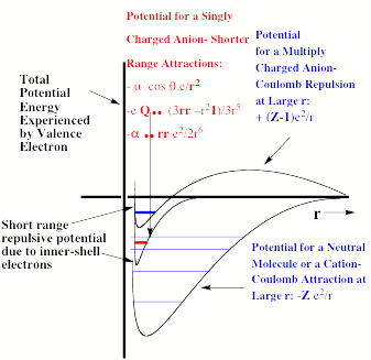
Figure 1.1. Plots of potentials experienced by valence electron in neutrals and cations, in singly charged anions, and in multiply charged anions.
In addition to these differences in long-range potentials, there are also qualitative differences in the inner valence-range potentials appropriate to anions, neutrals, and cations. Specifically, an electron in any molecule or ion containing N total electrons experiences Coulomb attractions (-Sa Zae2/|r-Ra|) to each nucleus (having charge Za); the total of such attractive charges is Ztot = Sa Za. This same electron experiences repulsive Coulomb and exchange interactions (e.g., given as a sum of Coulomb Jj and exchange Kj operators Sj=1,N (Jj – Kj) within the Hartree-Fock approximation that I will discuss in Chapter 2) with a total of N-1 other electrons. However, as Fig. 1.1 suggests, the balance between these Ztot attractions and N-1 repulsions is very different among neutrals, singly charged anions, multiply charged anions, and cations.
For a singly charged anion, Ztot = N-1, so, as noted above, there is no net Coulomb attraction or repulsion in regions of space where the electron-electron Coulomb and exchange terms cancel the nuclear attraction terms (e.g., for large r). However, in regions of space where this cancellation is not fully realized (e.g., within an oxygen p orbital of SO42- or inside the lone-pair orbital of the H3C- anion shown in Fig. 1.2 where the extra electron is not entirely shielded from the carbon nucleus by the other electron occupying this same orbital), a net attraction occurs. It is this net attractive potential and the fact that it has no long-range Coulomb character that ultimately determines the orbital shape and radial extent as well as the binding energy for the singly charged anion's extra electron.
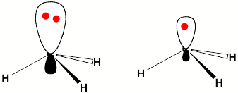
Figure 1.2. Doubly occupied orbital in the H3C- anion (left) and singly occupied orbital of the CH3 radical (right).
Note that the singly occupied orbital of the CH3 radical is drawn in Fig. 1.2 as being radially more compact than the corresponding doubly occupied orbital of the anion. This difference is size is due to the fact that the electron occupying the orbital in the neutral does not experience a Coulomb repulsion from a second electron in this same orbital (as occurs in the anion) and, as a result, this electron experiences a more attractive potential within the valence-orbital range and at large-r where the potential is of the attractive Coulomb form.
In contrast, for a neutral molecule or cation, Ztot is larger than N-1, so there exists a net Coulomb attraction at long range, as well as valence-range net attractive potentials, and repulsive potentials at even shorter range (due to repulsion from inner-shell electrons). The fact that the same kind of valence attractive potentials as in the anion are augmented by a long-range Coulomb attractive potential gives rise to stronger electron binding and smaller radial extent in such cases. For this reason, the minima in the potentials shown in Fig. 1.1 for the neutral and cation, are usually (i.e., for commonly realized values of the dipole moment, polarizability, etc.) deeper than for the anion cases. As a result, ionization potentials (IPs) of neutrals or of cations [[15]] usually exceed electron binding energies in anions (alternatively, electron affinities EAs of the corresponding neutrals [[16]]). This difference in the range of magnitudes of EAs and IPs is one of the most problematic facts for the theoretical study of anions. Specifically, any theoretical method that is able to produce electronic energy differences to an accuracy of 0.5 eV can prove valuable for studying IPs, which are usually significantly greater than 0.5 eV. However, many EAs are comparable to or less than 0.5 eV, so such theoretical predictions are of much less value for anions.
It is important to stress another attribute of the -1/r character of the attractive Coulomb potential appearing in neutrals and cations. As noted briefly earlier, when combined with the 1/r2 dependence of the electronic kinetic energy operator (-h2/2m∇2), the –1/r Coulomb potential gives rise to the well known Rydberg series of bound electronic states whose energies vary with quantum number n as –R/(n-d)2 (R being the Rydberg constant equal to 13.6 eV and d the quantum defect parameter embodying the effects of inner-shell electrons' repulsions). Anions do not possess the same kind of infinite series of bound electronic states because their long-range potentials vary as higher powers of 1/r. In fact, anions in which the excess electron is bound in a valence orbital (e.g., H3C- or HO-) have only one bound state rather than the infinite progressions of bound states that arise in neutrals and cations. On the other hand, anions with large dipole moments (> ca. 2 Debyes) can also bind an electron via their charge-dipole potential, but, unless the species has an extremely large dipole moment, only one electronic state is significantly bound (i.e., bound by > 100 cm-1). So, again, one does not observe an infinite progression of substantially bound states when dipole binding is operative; usually only one weakly bound state is seen. The bottom line is that one should not expect a molecular anion to possess any significantly bound excited electronic states; some anions have a few bound excited states, but most do not. The lack of bound excited electronic states presents significant difficulties for using spectroscopic tools to probe anions because such tools (e.g. laser induced fluorescence (LIF), resonance-enhanced multi-photon detachment (REMPD)) often rely on access to a bound excited state.
It is very important to be aware of the patterns of bound electronic states that occur in cations and neutrals and the paucity of bound states that characterize anions because one can not depend on the existence of an experimentally accessible progression of bound excited states to probe the electron detachment thresholds of anions as one often uses Rydberg series to approach ionization thresholds of neutral species. Moreover, the kind of vibration-induced electron detachment [[17]] processes that take place in Rydberg states of neutrals (in which a sequence of vibrational energy losses is accompanied by a series of Rydberg-state electronic energy gains) cannot occur in molecular anions. The anions do not have such a series of electronic states that can accept the sequence of vibrational energy losses and thus effect electron detachment, so one must use a different theory [[18]] to model such processes. In particular, the theory must allow for the anion to accept, in a single transition, enough vibration-rotation energy to undergo a bound-to-free transition in a single step.
For multiply charged anions, yet another situation arises since Ztot is smaller than N-1. As a result, at long range a repulsive Coulomb potential is operative. However, in the valence regions near the nuclei of the constituent atoms, the nuclear attractive potentials may be strong enough to overcome electron-electron Coulomb repulsions in certain regions of space (e.g., near the oxygen centers in TeF82-). In those regions, an electron may experience a net attractive potential that may be strong enough to bind the electron in which case the net potential will have the form shown in the upper part of Fig. 1.3 and one can have an electronically stable di-anion. Alternatively, if the valence-range attractive potentials are not strong enough to overcome the Coulomb repulsion, a potential such as in the bottom of Fig. 1.3 can result. In this latter case, a metastable state of the multiply charged anion may result (as in SO42-). In such a state, an extra electron can undergo autodetachment by tunneling through what is called the repulsive Coulomb barrier (RCB).
In both cases, one observes the RCB within which a bound or metastable state may exist. It should be noted that the long-range Coulomb repulsion that is operative in multiply charged anions has both destabilizing and stabilizing effects. The internal Coulomb repulsions certainly reduce the intrinsic electron binding potential of the shorter-range attractive potentials. However, the Coulomb repulsion also produces the long-range barrier that acts to confine or trap the electron; this confinement is especially important to consider when the multiply charged anion is metastable rather than electronically stable and thus susceptible to autodetachment. As we will see in Chapter 5, the RCB can cause multiply charged anions that are adiabatically quite unstable to have lifetimes exceeding seconds or minutes thus rendering them very amenable to detection and characterization.

Figure 1.3. Effective radial potentials experienced by the outermost electron in a doubly charged stable (top) and metastable (bottom) anion.
Of course, in a real multiply charged molecular anion the poential is not angularly isotropic; that is, it depends on the direction an electron moves as it attempts to escape. Two more quantitative representations of such potentials for doubly charged anions are shown in Figs. 1.4a and 1.4b. The former describes the potential experienced by the second excess electron in a linear structure of C62- [[19]] while the latter shows the corresponding potential in the tetrahedral species N(BF3)42- [[20]] with the potential plotted for a direction along one of the N-B bonds. In both cases, the potential is defined as zero when the second excess electron is infinitely far from the corresponding mono-anion.
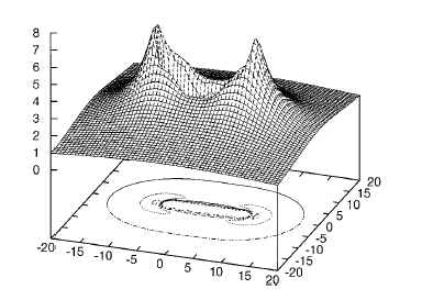
Figure 1.4a. Potential experienced by second excess electron in C62- with the molecule's center being located at (0,0) in the figure [19].
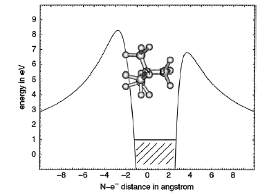
Figure 1.4b. Potential experienced by second excess electron in N(BF3)42- with the nitrogen atom being located at (0,0) and the molecule oriented as shown [20].
The examples shown in Figs. 1.4 illustrate that, although the Coulomb interactions between the two excess electrons produce a repulsive Coulomb barrier, the height of this barrier is not equal in all directions. This means that the second excess electron will escape by tunneling (when it is metastable with respect to a free electron and a mono-anion) with a highly anisotropic angular distribution. That is, the electron will be ejected preferentially in directions where the barrier is low and/or narrow and thus where tunneling is most favorable. Another implication of this observation is that, when carrying out theoretical studies on such dianions, one can obtain a reasonable estimate of the tunneling lifetime if one identifies regions where the Coulomb barrier is small and thin and computes (as an approximation) tunneling rates in such regions.
The differences in long-range and valence-range potentials experienced by the electrons produce some of the most profound differences in the physical and chemical properties of singly charged anions, multiply charged anions, and neutrals or cations. On a qualitative level, the fact that a Coulomb attractive potential, even with Z=1, is longer range (i.e., falls off as a lower power of 1/r) than charge-dipole, charge-quadrupole, or charge-induced-dipole potentials and produces a deeper well (i.e., for typical values of m, Q, and a found in typical molecules) than do the other potentials causes IPs to usually be larger than EAs. This in turn causes the sizes (i.e., radial extent of the outermost valence orbitals) and polarizabilities of anions to be larger than those of neutrals or cations of the same parent species. Moreover, these differences in potentials make the pattern of bound states very different for anions (i.e., few if any significantly bound excited states) than neutrals or cations (i.e., the infinite Rydberg progression of states as well as bound valence-excited states).
Also, as noted above, the Coulomb repulsive potential that occurs in multiply charged anions causes many such species to be metastable with respect to electron detachment or with respect to bond rupture (which subsequently produces Coulomb explosion as we will discuss in Chapter 5). For example, gas-phase (i.e., isolated) SO42, CO32-, and PO43- are not stable with respect to loss of an electron; these multiply charged anions undergo rapid autodetachment [[21]] in the gas phase. Only when strongly solvated (e.g., in aqueous solution or in the presence of several solvent molecules) are such multiply charged anions stable with respect to electron loss. In contrast, dicarboxylate dianions –O2C-(CH2)n-CO2- in which three or more methylene units separate the two anion centers are both electronically stable (i.e., neither excess charge spontaneously departs) and geometrically stable with respect to bond rupture and Coulomb explosion [[22]]. The primary difference between the SO42, CO32-, and PO43- and –O2C-(CH2)n-CO2- cases is the distance between the two or three excess charges, which, in turn, governs the strength of the repulsive Coulomb barrier. In the former three cases, the charges are too close to produce electronic stability (as in the bottom of Fig. 1.3). In the latter (at least for n ³ 3)), the distance between the two negatively charged sites is large enough to not render the dianion metastable.
Finally, it is worth mentioning how the differences in large-r potentials and subsequent differences in radial extent and electron binding energies can provide special challenges to the theoretical study of singly and multiply charged anions. In particular, when studying anions, it is important to utilize a theoretical approach that
- properly describes the large-r functional form of the potential (as we discuss in Chapter 2, not all commonly used quantum chemistry tools meet this criterion), especially for anions with very small EAs for which significant electron density exists at large r;
- is accurate enough to produce EAs of sufficient accuracy (this usually means that electron correlation effects must be included as we discuss in Chapter 2); and
- is capable of treating electronic metastability when the anion is not electronically stable (this is very difficult to do and is not a feature of most commonly used quantum chemistry software; we treat the special tools needed in such cases later in Chapter 5).
For singly charged anions in which the excess electron is bound tightly in a valence orbital (e.g., in F-, and organic RO-, RNH-, RCOO- anions), special atomic orbital basis sets are often not essential because the large-r amplitude of the anion's wave function is small. That is, most of the excess electron's density exists in the valence-orbital region. Such anions can be handled with the same kind of theoretical tools that have proven most useful in treating neutrals and cations.
However, when treating anions with very small electron binding energies, and thus large radial extent (e.g., dipole-bound anions such as NC-CH3-, (HF)n-, and NCH-), using an accurate method (because the EA is so small) and one that is proper at large r (i.e., contains charge-dipole interaction of a correct magnitude and no net Coulomb attraction) is important. In addition, using accurate methods that are correct at large r and which can handle metastable states is important when dealing with multiply charged anions. As discussed in Chapter 2, not all theoretical methods fulfill the criteria detailed above for use on weakly bound anions or multiply charged anions. In particular, most commonly used density functional theories (DFTs) contain potentials that do not behave properly at large r, although efforts are being made to remedy this [[23]]. In particular, most functionals contain an attractive –c/r Coulomb-type potential at large r, which clearly is not appropriate when treating such anions.
II. Anions Are Difficult to Prepare, Control, and Study as Isolated Species
A. Making Anions
The fact that most anions (and multiply charged anions) bind their outermost electrons less tightly than do most neutrals or cations contributes to the significant experimental difficulty one has in making substantial quantities of anions. Simple collisional attachment of an electron to a molecule M having a positive EA to form the anion M- is often not a fruitful means for preparing M- in gas-phase environments. Because the electron-attachment process is exothermic, and because total energy must be conserved in any binary collision, it may be impossible to form the stable ground state of M- directly in such gas-phase experiments. One needs to have some way to remove the excess energy (i.e., the exothermicity) released in forming M-. Moreover, as was emphasized earlier, because most anions do not have progressions of significantly bound excited electronic states, electron capture into an excited state, followed by radiationless relaxation to the ground state of M- is also not feasible. Thus, unlike cations C+, for which electron capture into a Rydberg state C**
C+ + e →C** → C,
followed by radiationless relaxation to lower states, is often an effective means of production of the neutral C, the analogous avenue is infrequently available to generate anions.
In contrast, dissociative electron attachment, followed by fragmentation to yield a fragment anion, is a commonly employed tool for forming molecular anions. In this process, an electron initially attaches by entering (usually) an antibonding orbital of the parent neutral molecule M-X:
M-X + e → (M-X)-*
to form a metastable state of the anion (M-X)-*. This state is metastable because the reverse process, autodetachment to return to M-X plus a free electron, remains possible so the (M-X)-* anion has a finite lifetime. There is a long and rich history of the experimental [[24]] and theoretical [[25]] study of such electronically metastable anions. These approaches provide some of the most direct data on antibonding molecular orbitals (e.g., in the e- + H3CS-SCH3 → (H3CS-SCH3-)* → H3CS- + SCH3 process, the electron enters an S-S antibonding s* orbital) and, as we emphasize here, they offer a good way to create a negative ion. Subsequent to such attachment, a fraction of the (M-X)-* species undergo bond rupture to form fragments M and X – before electron detachment from M-X-* occurs:
M-X-* → M + X-.
Of course, the amount of X- formed depends on the rates of fragmentation and of autodetachment. Often the latter rate is very fast (e.g., 1013--1014 s-1 or faster) and thus severely limits the yield of X- because fragmentation must take place on a timescale over which the M-X bond can appreciably elongate. The fragmentation is driven by the fact that the extra electron entered an antibonding orbital of M-X. Many anions have been generated by this kind of dissociative electron attachment processes in the gas phase using electron beams or electric discharges.
There are other avenues for forming molecular anions that are also commonly used. Once one has a source of one anion (say X-), one can generate other anions Y- by chemical reaction. For example, reactions of the type (R represents an organic functional group)
X- + R-Y → Y- + R-X
X- + H-Y → X-H + Y-
can be used when they are exothermic and proceed with no barrier. For example, the anion of a strong acid H-Y can be formed by reacting H-Y with the anion X- of a weaker acid H-X. Such reactions can also be used to, for example, rank order acid strengths; if X- does not abstract a proton from H-Y to form H-X + Y-, then HX must be a stronger acid than HY.
Another technique for generating anions is to collide the parent neutral M with a highly excited (often Rydberg) atom or molecule R**. A key to the success of such an approach is to find an excited state R** for which the energy required to remove its outermost electron matches the electron affinity of M, so that the process
M + R** → M- + R+
is thermo-neutral (or nearly so), in which case we say the electron transfer event is in resonance. Such resonance electron transfer collisions have especially high cross-sections (both because the Rydberg orbitals usually employed are spatially large and because of their energy resonance) and thus offer a good means for generating significant amounts of the desired anion. The groups of Professors Jean Pierre Schermann and Charles Desfrançois and Bob Compton have made [[26]] much use of this technique for creating a variety of anions including dipole bound anions (we discuss them in Chapter 4) by colliding a Rydberg atom with a highly polar molecule. In fact, the former workers have even been able to determine [[27]] the electron binding energy of the dipole-bound state thus formed by measuring the dependence of the cross-section for anion formation upon the principal quantum number of the Rydberg atom used to effect the electron transfer.
To form certain anions, one can use so-called laser ablation techniques. Here, one impinges a laser, whose photon energy hn and intensity can be controlled, onto a sample (usually a solid) of the material to be ablated. The ablation process causes fragments of the material to enter the gas phase with some of these fragments also undergoing ionization to form anions and cations. For example, a piece of solid aluminum subjected to laser ablation can generate Al, Al-, Al+, and various Aln-, Aln, and Aln+ cluster species. The size- distribution of the fragments will depend on the laser characteristics (fluence and energy), which are usually tuned to optimize production of the most desired species. In any event, the output of such a laser ablation ion source contains neutrals, cations, and anions of various cluster sizes. Because the anions are charged, mass spectrometric methods can then be used to select the species of the desired charge-to-mass ratio and to guide the anions into a reaction or spectroscopic-observation region.
There are several other approaches that one can use to form gas-phase samples of molecular anions. Because the intention here is to offer a brief introduction to some of the difficulties that arise in experimental studies of anions rather than to review all possible means of forming anions, we will not go further into this subject now. Instead, let us turn to focus on other aspects of the experimental studies.
When one is faced with forming multiply charged anions, special challenges arise, and another type of ion source is often used to overcome these difficulties. The so-called spray techniques are often used to form gas-phase samples of multiply charged anions (n.b., these sources can also be used to form singly-charged anions). Professor Lai-Sheng Wang's group has many papers in which these techniques are described in detail. In these methods, one typically begins with a liquid-phase sample containing the desired anion (usually existing in a strongly-solvated and hence highly stabilized state). One then injects a burst of the liquid sample into the gas-phase within the source region of, for example, a mass-selection device that we will discuss in the following Section. Injection is effected by using one of several spray techniques (e.g., electrospray, thermospray, etc.). As a result, one forms a gaseous sample containing
- solvent molecules S and perhaps solvent ions;
- the anion or multiply charged anion of interest M-n;
- the M-nspecies clustered with various numbers of solvent molecules MSK-n.
- other ions and solvated ions.
Many of the ion-solvent clusters formed in the initial spray event subsequently eject one or more solvent molecules losing mass and undergoing cooling in the process. This solvent evaporation process assists in producing internally (i.e., vibrationally and electronically) cold ion samples that can be mass-selected and subjected to subsequent reactions or spectroscopic examination.
As is the case with most techniques used to create molecular anions, the initial source preparation usually produces a complex mixture of ions that must be identified and selected to choose the particular ion whose behavior is to be examined. A mass spectrum of a sample derived from NH3 and H2 is shown in Fig. 1.5.
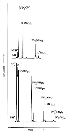
Figure 1.5. Intensity (vertical axis) of anions having various masses (horizontal axis) produced in a mixture of H2 and NH3 illustrating how various anions are usually identified and mass selected [256].
Clearly, there are many different negative ions in the gaseous sample whose mass spectrum is shown. If, for example, one were interested in studying H-(NH3) in a subsequent spectroscopic or reaction event, one must subsequently subject this sample to a mass-selection process to extract and control the desired anion.
For those readers who wish more up-to-date overviews of how molecular anions are formed in laboratory settings, there is a very recent review of electron affinities by Professors Barney Ellison and Fritz Schaefer [14]. Professor Ellison is one of the leading experimental figures in this rapidly expanding field; his contribution to that review provides the reader with much insight into how experiments on anions are carried out. That review also offers a wonderful avenue to much of the earlier experimental and theoretical studies of atomic and molecular electron affinities.
B. Selecting Specific Anions
Once an anion has been formed, it can be selectively removed from the source chamber using mass spectrometric, including ion cyclotron resonance (ICR), tools which rely on bending the trajectories of the various ions into arcs whose radii depend on the ion's charge-to-mass ratio. Let us discuss some of the basic physics involved to illustrate.
An ion of charge q and mass m moving with velocity v interacting with a magnetic field B experiences a Lorentz force directed perpendicular to the ion's velocity and perpendicular to the magnetic field
FL= q v x B.
This force has no component along the magnetic field direction (z), so the ion's motion along z is unperturbed. Within the x, y plane, any radial component of the ion's velocity experiences a torque and any angular component of the ion's velocity experiences a radial force. The outward-directed (i.e., radial in the x, y plane) centrifugal force FC generated by having the trajectory bent is
FC = m v2/r
where r is the instantaneous radius of curvature of the trajectory and v is the magnitude of the ion's velocity in the x, y plane. When the radial Lorentz and centrifugal forces come into balance, a stable circular orbit of radius
rstable = m v/(qB)
is formed. Once such a stable orbit is formed, the ions will move along the direction z of the magnetic field with unchanged speed vZ and will undergo periodic circular motions in the x,y plane perpendicular to B with a speed v that is unchanged. The force no longer change the speed (v = |v|) of the ion because the work
W = ∫ F•dr
done on the ion by this force is zero because F is always perpendicular to the trajectory's (angular) motion and hence no energy is imparted to the ion.
This shows that ions having mass-to-charge ratios m/q will, in the plane perpendicular to B, evolve into circular trajectories of different radii; the frequency n with which ions of a given q/m ratio move around these circular orbits is given by
n = (2p rstable/v) = (2p/B) (q/m).
This analysis suggests that, if one has a mixture of ions having different q/m ratios and a distribution of velocities (both v in the x,y plane and vZ along B), the ions will move unperturbed along the direction of B (i.e., with whatever speeds vz they initially possessed) but will be distributed in a series of circular orbits about the magnetic field direction. Although all ions of a given q/m ratio will have identical circular orbit frequencies, the radius of each ion's orbit will depend on the speed v in the x, y plane with which the ion began its motion (n.b., as mentioned above, this speed is conserved). If one wants to separate such a mixture of ions according to their q/m ratios, one could achieve spatial (i.e., radial) separation if one could force all of the ions to have the same speed.
To illustrate how one might achieve velocity selection, consider (it is illustrated for positive ions but the analysis also holds for anions) the crossed magnetic B and electric E field setup shown in Fig. 1.6.
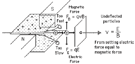
Figure 1.6. Illustration of a velocity-selection experimental setup.
Ions entering the magnetic and electric field region and having the dominant component v of their velocities lying along the direction perpendicular to both B and E will experience two forces of magnitude:
FB = q v B
and
FE = q E.
These two forces will oppose one another (in the direction of the electric field) and will thus deflect the ions' trajectories except for those ions whose velocities v happens to match
v= E/B.
These ions will not be deflected and thus will pass through this so-called velocity (or Wien) filter. By adjusting the E/B field ratio, one can then tune the ions' speeds if needed and one can guarantee that only ions of the same speed exit the filter.
The above analysis shows how one can bend trajectories of ions and make them undergo periodic orbiting motions whose frequencies depend on the q/m ratios and how one can velocity select ions. Now, let us explain the basics of how many mass spectrometers function. Most instruments, after ion formation, first subject all ions exiting the source to an accelerating electric field through which the ions undergo a potential change V. This causes them to gain kinetic energy by an amount
½ m v2 = q V.
If the accelerating potential is high enough, this kinetic energy will vastly outweigh any (e.g., thermal) kinetic energy the ions may have had prior to being accelerated. So, it is safe to assume that v given above is the total speed of the ions of mass m and charge q after they have been subjected to this acceleration. Solving for the speed v in terms of the potential V and substituting into the expression for the stable periodic orbit of radius rsstable, we obtain
m/q = B2 rstable2 /(2V).
Thus, if one accelerates all ions in a sample through an electric field of potential V and then subjects them to a magnetic field B, the different (i.e., having different m/q) ions' trajectories will be bent into orbits of different radii. So, if one has a way to sample the ions that are moving in the magnetic sector at a radius rstable, one will sample ions of a fixed m/q ratio.
Now, consider what happens if one has an instrument that passes a sample of ions through an accelerating electric potential V into a magnetic field region that has entry and exit slits that happen to be connected by a circular path of radius r0 as sown in Fig. 1.7.
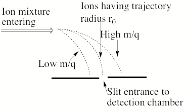
Figure 1.7 Schematic diagram showing ions of different m/q ratios bending with different curved trajectory with ions having radius r0 being selected to enter the detection chamber.
Then only those ions having m/q values given by
m/q = B2 r02/(2V)
will strike the exit slit and thus exit the magnetic sector to be detected in the next region of the instrument. However, by scanning the magnetic field strength B, one can cause ions of various m/q ratios to strike the exit slit and to thus be subject to detection. If one were to use a velocity filter containing electric and magnetic fields of strengths ES and BS, respectively, prior to injecting the ions into the mass-selection magnetic sector (of filed strength B), an ion having a given m/q ratio would be bent into an arc of radius
r= m v/(qB)
and its velocity would be given by
v = ES/BS.
So, the ions would move as shown in Fig. 1.8, and a detector placed on the outside of a slit at a distance r* could be used to detect ions of a selected m/q ratio by scanning the magnetic sector's field strength B until those ion's r value matched r*.
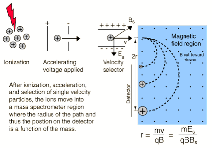
Figure 1.8. Schematic of mass spectrometer set up with velocity selection prior to injection into the magnetic sector.
Another example of a mass spectrometric ion-selection and detection apparatus that performs such tasks is shown in schematic form in Fig. 1.9. Such devices usually have several components including:
- A source region (on the left) in which the anions are formed.
- A region proximal to the source where electric fields are used to separate neutrals, positive ions, and anions and to accelerate and focus the anions (to the right in the Fig. 1.9);
- In the region where the anions are accelerated from left to right, a series of so-called electrostatic lenses are used to focus the anion beam onto a slit or pinhole opening in the next sector of the instrument.
- A magnetic sector within which the an electric field and a perpendicular magnetic field act to bend the anions' trajectories into circular arcs whose radii depend on their charge-to-mass ratio and to thus mass-select the ions;
- A region, subsequent to the mass-selection sector, where the anions whose radii of motion cause them to strike the entrance slit or hole of this region are collected (other anions strike the walls and are thus eliminated).
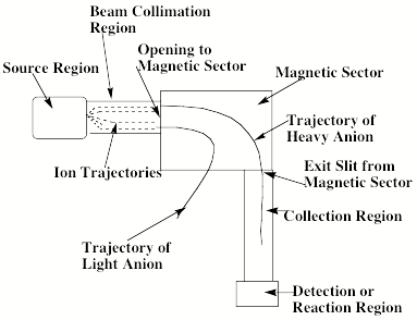
Figure 1.9. Schematic drawing of a mass-selection and detection device.
In the latter region, the mass-selected anion beam can, for example, be crossed with a photon beam to carry out photoelectron spectroscopy experiments. Alternatively, the beam can impact another beam (containing neutrals or other ions), a chamber containing a gaseous sample of other species, or a surface on which other species reside. Such impacts may then result in reactions whose products may be monitored using photon absorption, fluorescence, or mass spectroscopic techniques. More about these spectroscopic and reaction probes will be said in Sections IV and V of this Chapter.
An example of data obtained in a photoelectron spectroscopy experiment carried out on mass-selected ions is offered in Fig. 1.10 where the mass selection has allowed the workers to focus on the copper dimer anion.
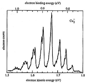
Figure 1.10. Photoelectron spectrum of Cu2- in which the number of electrons ejected as a function of the kinetic energy of the ejected electrons is plotted.
In such photoelectron experiments, a fixed-frequency light source shines on the mass-selected anion sample and the number of ejected electrons per unit time is monitored as a function of the kinetic energy of the ejected electrons. As Fig. 1.11 illustrates, the spacings between the peaks in Fig. 1.10 relate to the vibrational spacings of the neutral molecule produced when the electron is detached. Also, the photon energy hn minus the kinetic energy of the electrons ejected in the v=0 v=0 peak (if one can properly identify this) gives the adiabatic electron binding energy:
BE = hn - KE(0,0).
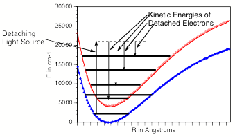
Figure 1.11. Anion (lower) and neutral (upper) potential surfaces with transition induced by absorbed photon and kinetic energies of ejected electrons.
In addition, if hot bands (i.e., transitions originating from excited vibrational levels of the anion) are observed, their energy spacings can be used to determine the vibrational level spacings of the anion.
If the neutral molecule accessed by detaching an electron from a molecular anion has low-lying electronic states, it is also possible to also observe peaks (at lower kinetic energy of the ejected electron or, alternatively, higher binding energy) corresponding to such excited states. An example of such a case is the iron dimer anion Fe2- for which there are two low-energy electronic states of Fe2 spaced by ca. 0.6 eV; the spectrum of this anion is shown in Fig. 1.12.
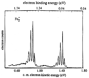
Figure 1.12. Photoelectron spectrum of Fe2- showing two sets of vibrational progressions, one for each of two electronic states.
The research group of Professor Carl Lineberger has, for many years, carried out such photoelectron experiments on atomic and molecular anions from which they have extracted many of the most up-to-date EA data on atoms, molecules and radicals, as well as vibrational level-spacing data on neutrals, radicals, and anions. The Lineberger group has also pioneered many of the experimental techniques used to form, select, and spectroscopically probe such anions. The group of Professor Kit Bowen at Johns Hopkins University has also carried out a large number of spectroscopic measurements on molecular anions to obtain the kind of information discussed above.
Another technique that relies on electric and magnetic fields to select and study ions according to their m/q ratios involves the ion cyclotron resonance (ICR) cell, which is illustrated in Fig. 1.13.
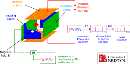 Figure 1.13. Schematic drawing of an ion cyclotron resonance cell.
A strong magnetic field B along the z-direction causes the ions to undergo periodic circular motions within the x, y plane as discussed earlier. The radius of such motion
r = (m/q) (v/B)
depends on the ion's m/q ratio and its speed v as well as the magnetic field strength B. For an ion with m/q near 100 Daltons moving at room-temperature thermal speeds and a magnetic field of 7 Tesla, the radius is ca. 4 x10⁻² mm. The frequency of this orbiting motion
n = 2 p B (q/m)
will be ca. 1 MHz under these conditions and thus be in the radio frequency (RF) range. In addition to the magnetic field along the z- axis, the ICR cell has two so-called trapping plates located at z = -L and z = L (z = 0 corresponding to the center of the cell) between which an electrostatic potential with spatial dependence of the form
V = ½ VT + ½ k z2
is applied. This potential exerts a force
FZ = - k q z
on the ions along the z-direction that acts to constrain the ions near the center of the cell (z = 0). In fact, this trapping electrostatic potential causes the ions to undergo harmonic motion along the z-axis of frequency
nz = 2p(kq/m)1/2
that depends on the m/q ratio of the ions.
So, in an ICR cell, the ions undergo periodic motions in the x, y plane of frequency 2pB (q/m) and along the z-axis of frequency 2p(kq/m)1/2. In Fig. 1.13 we also see two faces of the cell that are called excitation plates. If an RF field with a frequency matching the cyclotron frequency 2pB (q/m) of a group of ions were applied to these plates, energy would flow from this RF field and cause these ions to gain angular kinetic energy and to move into circular orbits of larger and larger radius. The coherence of this RF field would also cause the ions in resonance with it to move together coherently; prior to application of this field, all these ions moved with the same frequency 2pB(q/m) but their angular movements were not coherently coordinated. This group of ions moving coherently together will then induce a time-dependent image current in the detector plates shown in Fig. 1.13. If this current is measured and digitized, the signal can be Fourier transformed and, not surprisingly, will produce a frequency spectrum with one component n= 2pB (q/m).
If, instead of applying an RF field of one chosen frequency, one applied a broad-band RF pulse, one could resonantly and coherently excite the cyclotron motions of all (or at least for a wide distribution of q/m values) of the ions in the ICR cell. The motions of these ions would, in turn, generate a time-dependent image current in the detector plates. Upon digitizing this time-dependent current and Fourier transforming the resulting signal, one obtains a frequency spectrum with peaks at each of the 2pB(q/m) frequencies belonging to each group of ions in the cell. The intensity of each peak is proportional to the concentration of ions having the corresponding q/m values in the cell. In this manner, the ICR experiment can identify a wide range of q/m values using a single RF excitation pulse strategy in contrast to scanning the excitation frequency.
Before closing this Section dealing with mass (actually q/m) selection, it is important to mention a selection device that does not use magnetic fields at all. A so-called time-of-flight (TOF) mass spectrometer accelerates a mixture of ions through a potential drop V using an electric field. After exiting this acceleration stage, an ion will have a kinetic energy
½ m v2 = q V,
so its speed along the direction of the electric field (z) will be
v = (2 V q/m)1/2 .
These ions are allowed to undergo undisturbed (by collisions or fields) movement along the z-direction for a distance D at which position they are detected. The time t it takes an ion to reach the detection position is
t = D/v = D (m/q)1/2 (1/2V)1/2.
So, ions with small m/q values will reach the detector before ions with higher m/q values. By determining the times at which various ions reach the detector (so-called arrival times), one can thus determine their m/q values.
Professor John Brauman's group has pioneered the use of ICR methods to both separate and trap (i.e., contain for long times) ions of a chosen mass to charge ratio. As we will discuss in Sec. V of this Chapter, chemical reactions can also be carried out within the ICR cell and the appearance of product ions, having different q/m values, can be monitored using the above ICR methods.
By injecting radiation into the ICR chamber that is resonant with ions having qJ/MJ, one causes such ions to be ejected from the chamber. One can thus eject all ions but those whose q/M ratio corresponds to the desired ion. These mass-selected anions then undergo circular motion in the ICR source until collisions or radiation causes them to change trajectory and thus be eliminated. Trapping times in the seconds or minutes range are not uncommon in such experiments. One of the main advantages of an ICR source is the long time that one can trap ions for subsequent study. For example, if one wishes to probe the infrared (IR) absorption or emission of anions, it is useful to have the ions within the spectral regions for long times because IR absorption and emission rates are quite low. The ICR chamber can also be used as a region where photodetachment or chemical reactions of the selected anions occur. That is, as the anions circulate throughout the ICR chamber, they can be subjected to radiation or to collisions with other reagents and the outcomes (i.e., ejected electrons or production of reaction product ions) of such processes can be examined.
It is possible to use the same kind of physics just discussed to bend and accelerate ions not into small circular orbits but into large paths (i.e., several meters in diameter) that constitute a storage ring. The groups of Professors Torkild Andersen and Lars Andersen in Aarhus have used such instruments to create, store, and study spectrocopically a wide variety of molecular anions.
C. How Fields Are Used to Focus and Select Anions
As shown in Fig. 1.9, when ions leave the source region, it is often found useful to arrange for them to be spatially directed before they enter, for example, a velocity selection or mass separation region. This step allows one to cause a larger fraction of the ions produced in the source region to be used in the experiment. It is theefore instructive to discuss how the collimating and collection sectors shown in Fig. 1.9 operate. In the latter, the (usually cylindrical) tube that forms this sector has several rods arranged symmetrically about its outer edge. For example, if one were to view this sector looking down the length of the tube, one would see what is qualitatively depicted in Figure 1.14 where octopole (left) and quadrupole (right) arrangements appear.
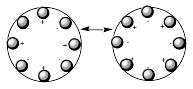 Figure 1.14. Time varying positively and negatively charged octopole rods (left) and
rods in a quadrupole arrangement (right).
Figure 1.14. Time varying positively and negatively charged octopole rods (left) and
rods in a quadrupole arrangement (right).
Various numbers of rods can be employed; many rods as in the left of Fig. 1.14 produce a field near the center of the circle that is flat bottomed as that shown in the left of Fig. 1.15, while few rods as in the quadrupole on the right of Fig. 1.14 give a field like that shown in the right.
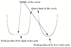 Figure 1.15. Radial constraining field for multipoles of high and low orders (top)
and trajectories of light ions (left), heavy ions (middle), and selected ions (right)
under combined RF and DC potentials.
Figure 1.15. Radial constraining field for multipoles of high and low orders (top)
and trajectories of light ions (left), heavy ions (middle), and selected ions (right)
under combined RF and DC potentials.
An instrument having 2N rods produces a radial constraining field that varies as 1/R2N-2, where R is the distance from the center of the circle. So, the octopole arrangement shown in Fig. 1.14 would produce a field varying with R as 1/R6 and a quadrupole produces a potential that is quadratic and varies as 1/R2 as in Fig. 1.15 on the right.
An anion located in the center of this circle and moving axially down the tube will experience no net force from the positive and negative charges of the rods. However, an anion located away from the center of this circle will experience a net force; it will be attracted to the positive rods and repelled from the negative rods. If the rods retained fixed charges, the anions would eventually strike a positive rod and be removed from the beam. However, when operated in a mode to guide an ion beam but not separate ions by q/m values, the rods' charges are alternated by application of an external alternating potential (usually in the RF range). If the period of this oscillation is short enough, an anion initially attracted to a positive rod will soon be repelled from this same rod (as it becomes negatively charged) and attracted to the oppositely charged rods. The net result is that an anion will experience a time-averaged field that varies with distance R away from the center of the circle shown in Figure 1.15. This potential acts to trap the ions radially. For a low-order multipole, it also acts to focus the ions toward the center of the cylinder, whereas the flat-bottomed nature of the higher order multipole's potential does not focus to such an extent but it still guides the ions down the cylinder.
Now, let's consider what happens if one applies both an AC and a DC field (VDC + VAC cos(wt)) to two opposite poles of a quadrupole while applying (-VDC - VAC cos(wt)) to the other two poles. The alternating electric field causes the ions move in spiral paths of larger and larger radial size as they pass down the quadrupole's long axis. The DC voltage acts to drag them in one direction, towards one pair of electrodes. A light ion will be dragged a large distance by the alternating field, and will quickly collide with an electrode and disappear as shown on the bottom left of Fig. 1.15. A heavy ion will not be deflected radially as much by the alternating field, but will be gradually pulled by the DC field as shown in the middle of Fig. 1.15 so it will also collide with an electrode, and be lost. In contrast, an ion that has just the right q/m will drifs slightly due to the DC field, but will be pulled back toward the center of the quadrpole by the AC field as long as the amplitude of the AC field is not large enough to make this ion spiral out of control into an electrode. Thus an ion just the right size is stable in this quadrupole field and reaches the end, where it can be measured. By scanning the magnitudes of the AC and DC fields, one can arrange for ions of a desired q/m value to be stable within the quadrupole filter. In this way, a quadrupole can act as a mass-selection device. In addition, by choosing the strength of the DC field to be stronger than that of the AC field, heavy ions will be pulled out of the center while the lighter ions will be stabilized by the DC field, so one can create a so-called high-mass filter. In reverse, by choosing the AC field to be stronger than the DC field, the light ions will be destabilized and thus ejected while the heavier ions will respond mainly to the DC field and have a better chance of passing down the quadrupole, thus creatng a low-mass filter. Finally, the use of multipole fields can also allow one to confine ions within a three dimensional region of space for long periods of time as in a so-called quadrupole (or Paul) trap. The American Association of Mass Spectrometry has a nice web site that explains how various mass-selection and ion-trapping devices work.
Let us now turn to our discussion of the collimating sector where a series of electrostatic lenses is used to both accelerate the anions (from left to right in Fig. 1.9) and to focus the ion beam toward the center so it can pass through an entrance hole or slit of the magnetic sector. The lenses often consist of a series of circular plates, such as shown in Fig. 1.16, with successive plates held at a higher voltage than the preceding plate.
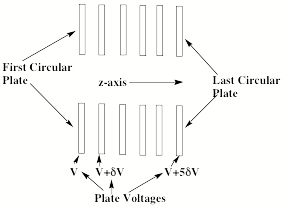 Figure 1.16. Series of plates constituting an electrostatic lens.
An anion moving from left to right down the z-axis of such circular plates will be accelerated because it experiences an electric field gradient. Such a gradient ∂V(z)/∂z produces a force Fz = - q∂V(z)/∂z along the z-axis (here q is the anion's charge) that acts to accelerate the anions.
A closer look at the electric fields within and between successive plate regions is shown in Fig. 1.17 for a pair of plates.
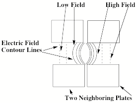 Figure 1.17. Electric field contour lines within and between two plates.
Because the force acting on an anion is proportional to the gradient of the electric field, this force is directed perpendicular to the contour lines of the electric field. At regions deep within a plate, the force is directed along the z-axis. However, in the regions between plates and extending somewhat inside each plate, the contours have the curved shapes shown in Fig. 1.17. The resultant field gradients produce forces that cause an anion to be moved inward toward the center of the circular plates. In this manner, the anions' trajectories are focused along the z-axis as they are accelerated along this direction.
D. Problems That Can Occur
A significant problem that arises in ion beam experiments relates to what is called space charge effects. When an ion beam is collimated and focused, the ions are forced close together and thus repel one another strongly. The Coulomb repulsion among the ions tends to resist the forces applied by external fields designed to collimate and/or focus the beam. As a result, it is very difficult to retain a tightly collimated and intense beam of ions even using the devices discussed above.
Another difficulty arises from the ability of any applied electric field to pull the excess electron(s) off the anion of interest. To understand how this field-detachment process works, consider the radial potential that an excess electron experiences when an external electric field of strength E is applied. In Fig. 1.18, we illustrate the two potentials that such an excess electron experiences- the potential intrinsic in the electron-molecule interaction and the potential due to the electron-field interaction.
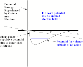
Figure 1.18. Long- and short- range potential experienced by excess electron (smooth curve) and potential E r cosq due to applied electric field.
The smooth curve is meant to describe the kind of potentials discussed in detail earlier in Section I of this Chapter (see Fig. 1.1), while the straight line describes the r-dependence of the charge-field potential - E r cosq due to the external electric field of strength E (q being the angle between the field direction and the spatial location vector r of the electron). Also shown in Fig. 1.18 is the energy of the bound state of the anion in the absence of the external electric field.
Of course, the excess electron moves under the influence of a total potential that is a sum of the charge-field potential and the potential operative in the absence of the field. In Fig. 1.19, this total potential is depicted (for two values of the field strength E and for q such that cosq is positive).
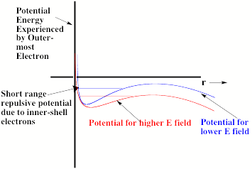
Fig. 1.19. Total radial potential experienced by excess electron in an anion in the presence of an external electric field.
The important thing to notice in Fig. 1.19 is that the total effective potential has a barrier beyond which the potential decreases as r increases. The form of this potential allows the attached electron to tunnel through it and thus undergo detachment. Of course, the lifetime of such an anion with respect to tunneling will depend on the binding energy and the strength of the applied field. The stronger the field, the lower is the barrier in the potential as shown in Fig. 1.19 and the shorter is the lifetime. In fact, if the field is strong enough, the barrier will occur at the energy of the electronic state and tunneling will not be required for the electron to escape. At this critical field strength, the electron can simply fall off the barrier.
To shed further light on the matter of field-induced detachment let us examine the case in which no (or little) tunneling is required for electron detachment. We begin by assuming that the long-range part of the potential shown above (in the absence of the external field) is of the form
Vlong-range = - A r-n.
Such an expression is consistent with the prototypical dipole, quadrupole, or polarization potentials discussed earlier as well as with the n = 1 Coulomb potential appropriate to neutrals and cations. Adding to this long-range attractive potential the electron-field interaction potential - E r cos q, we obtain the following total potential at large-r:
Vtotal = - A r-n - E r cosq.
Taking the derivative of this with respect to r and setting the derivative equal to zero (to determine the location and the energy of the barrier), we find:
rbarrier = (nA/Ecosq)1/(n+1).
At this value of r, the total potential is
Vtotal = - A[Ecosq/nA]n/(n+1) – Ecosq [nA/Ecosq]1/(n+1)
= - [nA/Ecosq]1/(n+1) Ecosq {1 + 1/n}.
Along the direction where cosq is largest (i.e., along which the field effect is strongest), the value of Vtotal at the barrier reduces to - [nA/E]1/(n+1) E {1 + 1/n}. For example, in the case of dipole binding (n = 2) Vtotal = - 3/2 (2A)1/3 E2/3. In comparison, for states of neutrals or cations for which the longest-range potential is the Coulomb potential (n = 1), Vtotal = -2A1/2 E1/2. The point of this analysis is to show that the barrier in the total potential lies below zero (i.e., below the detachment threshold) by an amount that varies as the 2/3 power of the applied electric field for dipole binding but as the 1/2 power of the electric field for the Coulomb potential, which relates to neutrals and cations, not anions. So, again, we see a qualitative difference in the behavior of anions and other species.
As noted above, as the applied electric field in increased, the barrier eventually reaches a level at which the bound anionic state (e.g., the level of the horizontal line in Fig. 1.19) becomes unstable. At such field strengths, the quasi-bound level no longer requires tunneling to effect electron detachment; the electron can simply detach by falling over the barrier. So, electric field detachment can cause problems if the applied field is strong enough to cause the anion to lose its electron(s) before its properties are studied.
Alternatively, the strength of binding of the excess electron(s) in an anion can be studied by subjecting the species to external electric fields of increasing strength, and determining at what value E of the field electron loss becomes very facile (i.e., when the barrier drops below the energy of the quasi-bound state). Indeed, this effect has become a powerful and widely used tool for determining electron binding energies, especially in species with quite small EAs.
Before closing this Section dealing with the problems that can arise when studying anions in the laboratory, we need to offer another note of caution. Even when utmost care is taken to optimize source conditions and carry out mass selection and extraction, one must keep in mind that the final anion sample may not contain only the anions that one has in mind. For example, imagine that one were to prepare a sample containing H- anions clustered with various numbers of NH3 molecules. After one extracts the anions from this sample and subjects them to mass selection (being careful to select only ions of mass-to-charge ratio of 18), one expects to have a beam of H- (NH3) anions. However, there may be other species in this beam!
For example, if the source contained any oxygen atoms, one may have OD- ions also present. This problem can be dealt with by realizing that OD- does not weigh exactly the same as H-(NH3) and that OD- has an electron detachment energy of ca. 1.8 eV, whereas H-(NH3) binds its electron by only 1.4 eV. For these reasons, one could either increase the resolution of the mass selection to permit only the desired H-(NH3) ions to enter the detection region, or spectroscopically probe for anions that detach below 1.8 eV.
However, another kind of problem is more difficult to handle- that of structural isomers. For the H-NH3 example at hand, one may have an appreciable amount of the double-Rydberg anion (we discuss such anions in detail later) NH4- that is an isomer of H-(NH3). NH4‑ consists of an NH4+ cation to which a pair of electrons is bound in a diffuse Rydberg orbital such as shown in Fig. 1.20. All molecular cations have such Rydberg orbitals because they possess a positive charge whose Coulomb potential can attract and bind at least one electron.
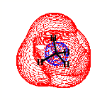
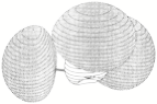
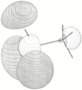
Figure 1.20. Rydberg orbitals of NH4+, H3O+, and H3C-NH>3+
One way to think of the NH4- anion is in terms of its isoelectronic analog, the Na- anion. If one thinks of taking the +11 nucleus of Na and splitting it into five parts- a +7 nucleus at the origin and four +1 nuclei placed tetrahedrally about the origin, one forms the nuclear geometry of NH4-. By then allowing the eleven electrons of Na- to move not in the spherical potential of a single +11 nucleus but in the presence of the five positive nuclei, one forms NH4-. So, Rydberg species can be viewed in terms of their united-atom isoelectronic analogs. It turns out that all molecular cations have Rydberg orbitals that can be thought of as arising from the attractive long-range Coulomb potential -e2/r combined with valence-range repulsive potentials from the Coulomb and exchange interactions with the cation's other electrons (e.g., the N 1s and four N-H bond pairs in the NH4+ example). It is these inner-shell electrons that cause the energy level patterns of Rydberg states to fit the –R/(n-d)2 pattern with a non-zero quantum defect d. Placing one electron into a Rydberg orbital of a cation generates a neutral Rydberg species such as NH4 whose electronic states can indeed be fit to such a formula. Placing two electrons into such Rydberg orbitals generates what is called a double-Rydberg anion such as NH4- about which I will have more to say in Chapter 4. Let us return now to discuss how such geometrical isomers can plague experiments.
If one were to assume that only H-(NH3) were present and, for example, carry out endothermic reactions of the mass-selected anion beam with reagents X for which formation of HX- + NH3 from X + H-NH3 were say 1.1 eV endothermic, one would obtain surprising results if an appreciable amount of the NH4- isomer were present. Because the double-Rydberg isomer lies 0.8 eV above H-(NH3) on this anion's ground-state energy surface, its reaction with X to give HX- + NH3 is exothermic by only 1.1-0.8 = 0.3 eV. As a result, when the anion beam is accelerated to a kinetic energy of 0.3 eV and allowed to undergo collisions with X, formation of HX- product ions would be observed. If one were to interpret this threshold for HX- production in terms of the DE for the reaction
H-(NH3) + X → HX- + NH3,
one would be incorrect. This threshold really related to the DE of the following reaction:
NH4- + X → HX- + NH3.
So, in addition to using mass selection, it may help to also carry out, for example, photoelectron spectroscopic probes of the reactant-ion sample to determine whether more than one isomer is present. In fact, it was precisely through such a careful examination of the photoelectron spectrum of H-(NH3) that Professor Kit Bowen discovered the double-Rydberg species (NH4)- that we have been discussing. The Bowen group has been active for many years studying such anion clusters as well as more exotic species (e.g., dipole-bound anions) discussed in Chapter 4 and biological-molecule anions treated in Chapter 7.
Finally, I want to mention one more difficulty that can occur in the kind of experiments outlined above. Again using the NH4‑ example, if one mass selects on M/q = 18, one may have some [(NH4)(NH4)]2- dianions present in addition to the desired H-(NH3). So, species that are dimers or higher oligomers of the species one is attempting to select can also be present in the mass-selected beam. All of the complications discussed above present serious challenges to the experimental chemist and, at times, make interpretation of experimental data ambiguous or, at least, very challenging.
The main point of the above examples is to illustrate that mass selection alone does not guarantee one has only one kind of anion in the beam that is thereby produced. One must always be aware of the possibilities of species with nearly identical masses and isomers and dimers (and other oligomers) of the species one wishes to study.
This concludes this overview of how anions can be made and subsequently selected according to their mass-to-charge ratio. Such mass-selected ion samples can then be subjected to, for example, spectroscopic probes or collisions with other species with which they might react. In the latter case, other product ions may be formed, so this reaction region would have to be equipped with an ion extraction and second-stage m/q detection region to probe the identities and abundances of these product ions.
III. Anions Experience Strong Environmental Effects
When an anion is surrounded by other molecules as in solution, in a cluster, at an interface, or in a solid matrix, it experiences very strong intermolecular potentials. Moreover, because anions' valence electron densities are typically more diffuse and less tightly bound than those of cations, the anions' outmost orbitals can interact more strongly with surrounding molecules. This does not mean that the solvation energies of anions exceed those of cations but that the valence orbitals of anions can be more strongly affected (e.g., their electron binding energies can be altered by a larger percent) by solvation.
To illustrate, a typical energy with which a single H2O or NH3 molecule is bound to a small anion such as F-, Cl-, or OH- is in the 20-30 kcal mol-1 range as are the corresponding ion-molecule interaction energies for K+ and Li+ (19 and 32 kcal mol-1, respectively). In H2O or NH3, the total solvation energies of each of these ions is larger than the energies [[28]] just quoted because solvation involves many ion-solvent and solvent-solvent interactions. In contrast to the strength of the ion-solvent interaction energies, the energy of attraction between a pair of H2O or of NH3 molecules is in the 3-7 kcal mol-1 range, and these hydrogen bonding solvents contain among the stronger attractive potentials that act between pairs of neutrals.
One of the most important influences of the large solvation energies that anions experience occurs in the electron binding energies of such solvated anions. Because the anion M- is more strongly than its parent neutral M, the M-→ M energy gap is significantly larger for the solvated species than for the gas-phase counterparts. As a result, the photoelectron spectra of solvated anions have their peaks blue-shifted (i.e., moved to higher detachment energies) compared to their gas-phase counterparts. Of course, analogous but smaller spectral shifts are observed when M- is partially solvated (e.g., as in M-(H2O)n cluster ions).
Differential solvation effects can also affect reaction rates and the energy profiles along reaction paths. For example, in the widely studied SN2 reactions such as Cl- + H3C-Br Cl-CH3 + Br-, the energy of the transition state [Cl—CH3—Br]- relative to that of the reactants and of the products is not the same in solution as in the gas phase. Hence, the activation energy and the forward and backward reaction rates are affected by solvation. Professor John Brauman's group has done more than any other to elucidate such solvation effects on reaction energy profiles for a wide range of organic reactions. The physical origin of solvent effects on such reaction profiles lies in the different solvation energies of the Cl- and Br- anions as well as of the transition-state anion. In particular, because the negative charge is delocalized over both halogen sites in the transition state, the solvation energy of this species is smaller than are the solvation energies of the more charge-localized Cl- and Br- ions. In Fig. 1.21 we illustrate these effects.
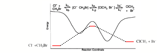
Figure 1.21. Energy profile for typical SN2 reaction in the gas phase (black) and in a strong solvent (red).
Because of the very large differential solvation of the charge-localized reactant and product ions, the energy of the transition state changes from lying below that of the reactants (i.e., in the gas-phase) to lying above the reactants (i.e. in solution). Hence, solvation can even qualitatively alter an ionic reaction's energy landscape.
The Brauman group has used ion-cyclotron resonance techniques coupled with gas-phase photoelectron spectroscopy to probe such reaction-path energy profiles for a very wide variety of important organic ionic reactions. By comparing their results to what was known earlier about the same reactions in solution, they have been able to clearly identify the roles of intrinsic (i.e., in the absence of solvation) electronic effects and those of solvation. Such studies have essentially revolutionized how we view many organic reaction mechanisms.
The substantial differential stabilization of the anion relative to the corresponding species with one fewer electron can even cause ions that are unstable with respect to spontaneous electron loss in the gas phase to become stable when solvated. For example, isolated (i.e., gas phase) SO4-2 and PO4-3 are not electronically stable; they spontaneously eject an electron to produce SO4-1 and PO4-2, respectively (PO42- even ejects another electron to give PO4-). However, when solvated by a few H2O molecules to form SO4(H2O)n-2 and PO4(H2O)n-3, these ubiquitous anions become electronically stable. Professor Lai-Sheng Wang has examined several such metastable anions and has focused proper attention on the role of solvation in stabilizing these species. The Wang group uses electrospray-type sources and so-called magnetic bottle methods to contain the selected ions for long times. They then carry out photoelectron spectroscopy experiments on these anions. Using such methods, they have been successful in studying a wide range of multiply charged anions and cluster anions including many metastable anions.
When anions are stabilized by surrounding solvent molecules, not only do their electron binding energies increase, but the radial extent of the outermost orbitals containing the excess electron(s) is also reduced. Of course, the two effects- an increase in binding energy and shrinkage in orbital size- go hand-in-hand, as they do for neutrals and cations. In fact, the functional form of the exponential decay that governs the radial extent of any orbital is related to the electron binding energy of that orbital as
exp(-r(2mDE/h2)1/2),
where the electron detachment energy (DE) is the energy needed to (vertically) remove an electron (with mass m) from that orbital. From this relationship, it is clear that species such as anions with small electron binding energies must have more diffuse (i.e., radially extended) electron distributions. The average value of the radius of such an orbital is given by
<r> = 3h/(2(2mDE)1/2),
which suggests how the radial size (of the outermost orbitals) depends upon DE.
IV. Spectroscopic Probes
Once the anions have been mass selected and extracted, they can be subjected to various probes. The two most common interrogations involve carrying out some kind of spectroscopy on the ions or allowing the ions to undergo reactive collisions with another gas (or with a solid surface) after which product ions' identities and abundances are determined. In this Section, we will discuss some spectroscopic studies that can be carried out. However, in Chapters 3-7 many more examples of spectroscopic and chemical reaction studies of molecular anions will be given.
The number density of anions that are available (after formation and mass selection) for spectroscopic study is often low because of space charge effects or because the anions may be difficult to make in significant abundance. Thus straightforward absorption-type spectroscopies in which one monitors the attenuation of the intensity of a photon beam and uses the Beer-Lambert law
log (I0/I) = e C L
to determine the ion's concentration C or to monitor the wavelength dependence of its extinction coefficient e are not feasible. There is just too little absorption to measure it accurately. Also, because molecular anions seldom have bound excited electronic states, methods such as laser-induced fluorescence (LIF) cannot be employed.
For these reasons, one must resort to so-called action-based spectroscopic methods to study molecular anions. In these approaches, one measures an outcome of light absorption that can be quantified with high sensitivity and resolution against a near-zero background signal. The simplest example, and one of the most widely used techniques involves photoelectron and photodetachment spectroscopies. In the former, one uses a fixed-frequency (n) light source (these days, most likely a laser) to eject electrons from a molecular anion source and then one measures (as the action) the appearance of emitted electrons whose kinetic energies KE one also measures. To increase the path length over which the anions are irradiated, it is useful to align the light beam coaxially to the ion beam.
For a transition in which an anion M- (e,v,J) in electronic state e, vibrational level v, and rotational level J ejects an electron to generate a neutral M (e',v',J') in its corresponding states, electrons will be detected with kinetic energies given by
KE = hn - {E[M (e',v',J')] – E[M- (e,v,J)]}.
If one is able to identify the peak (i.e., grouping of ejected electrons) corresponding to a transition from the ground e, v, J state of the anion into the ground e',v',J' state of the neutral, the adiabatic electron affinity (EA) can be determined from
EA = hn - KE0,
where KE0 is the kinetic energy of the electrons ejected for this peak. An example of a photoelectron spectrum for the DOO- anion [[29]] from the laboratories of Professors Veronica Bierbaum, Barney Ellison, and Carl Lineberger is shown in Fig. 1.22 where the intensity of ejected electrons is plotted as a function of the electron binding energy (BE) for each peak determined in terms of the kinetic energy of the electrons ejected in that peak as
BE = hn - KE.
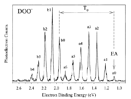
Figure 1.22. Number of photoelectrons as a function of electron binding energy for various vibrational transitions in DOO- → DOO + e-.
In ref. 29 the peaks labeled a0 through a6 were assigned to transitions in which the neutral HOO radical is formed in its ground X 2A'' electronic state with zero (a0) through six (a6) quanta of vibrational energy in the O-O stretching mode. Peaks b0 through b4 were determined to correspond to transitions in which HOO is formed in it's excited A 2A' electronic state with zero (b0) through four (b4) quanta of vibrational energy in the O-O stretching mode. Thus, the adiabatic EA can be determined from the energy of the a0 peak to be 1.08 eV and the electronic X → A excitation energy in HOO is given by the spacing between the b0 and a0 peaks to be 0.87 eV.
As in all spectroscopic work, determining what transition each peak corresponds to is difficult work. Of course, one looks for series of peaks whose spacings seem to fit a progression (i.e., become closer spaced due to anhramonicity as one moves to higher levels). However, if the geometry change accompanying electron ejection is large, there may be very low Franck-Condon factors connecting to the neutral's lowest vibrational level, so identifying the peak corresponding to transitions to this level. This limitation can make it difficult to evaluate the adiabatic EA. In addition, hot bands (i.e., transitions originating from excited vibrational levels of the parent anion) will produce peaks having low electron bininding energies and may further complicate the peak-assignment challenge.
The workers in ref. 29 used the EA data determined from the photoelectron spectrum to determine the enthalpy of formation of HOO (and DOO) as follows:
- In a separate reaction dynamics experiment, they determined DG298for the reaction
HOO- + HC ≡ C - H ⇆ HOO - H +HC ≡ C-.
- Knowing the gas-phase acidity DGacidof acetylene, they could determine the gas-phase acidity of HOOH from
DGrxn298 = DGacid (HCCH) - DGacid (HOOH).
- The gas-phase acidity of HOOH relates to the reaction
HOO-H → H+ + HOO-,
so one can obtain the DHbond for the homolytic bond cleavage
HOO-H → H + HOO
if one knows the IP of the hydrogen atom (which is very accurately known) and the EA of the HOO radical, which they determined in the photoelectron experiment. In this way, they were able to determine the enthalpy of formation of HOO by
DHf,298(HOO) = DHbond - DHf,298 (H) + DHf,298(HOOH),
using the known enthalpy of formation of HOOH, and obtained DHf,298(HOO) = 3.2 ± 0.5 kcal mol-1.
In Fig. 1.23 we show another example of a photoelectron spectrum [[30]] for the H3COO- anion also obtained by the Boulder team mentioned above.
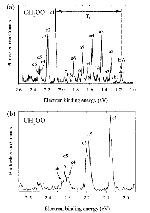
Figure 1.23. Photoelectron spectrum (a) of H3C-OO- showing several vibrational progressions and (b) a similar plot focused on the region of peaks c1-c6.
By determining that peak a1 corresponds to producing H3COO radical in its X 2A'' electronic state with no excess vibrational energy (from the corresponding anion in its lowest electronic and vibrational level), the workers of ref. 30 determined the EA to be 1.16 eV. Be determining that peak c1 corresponds to producing H3COO in it's A 2A' excited electronic state with no excess vibrational energy, they determined the X → A energy gap to be 0.91 eV. From these examples, we see how EA data and photoelectron spectroscopy provide data that is useful in determining energies of excited electronic states of radicals (formed by removing an electron from the anion) and in determining a wide range of thermodynamic data on such species.
In photoelectron spectroscopy (of anions and of neutrals), a limiting factor in how accurately electron binding energies can be measured is the ability to measure the kinetic energies of the ejected electrons. Typically, one can not measure electron energies better than ca. 0.03 eV, which, of course, means EA values can not be determined to better than this limit. By using the fact that the photon energy hn can be specified to much higher accuracy than the ejected electrons' kinetic energies can be determined, one can do better as we now discuss.
In threshold photodetachment spectroscopy one does not use a fixed-frequency laser. Instead one uses a tunable laser. By increasing the energy of the light source until one observes ejected electrons, one can determine the energy gap between the anion and the neutral. At higher photon energies, neutrals in excited (vibration-rotation or electronic) states can be produced, which one quantitates by looking for an increase in electron yield as hn increases (i.e., each such channel opening generates an increase in the electron ejection rate). A very important advantage of this approach is that one does not need to measure the ejected electrons' kinetic energy; all one needs to do is to detect the electrons that have been ejected. In this way, one can achieve spectral peak resolutions in the range of 0.003 eV, thus increasing the resolution compared to photoelectron spectroscopy by approximately an order of magnitude. An example [[31]] from Professor Dan Neumark's lab comparing photoelectron and threshold photodetachment spectra on IHI- is given in Figs. 1.24 and 1.25. In the former, the photoelectron spectrum is shown, while in the latter, the threshold photodetachment spectrum is shown near the v3' = 2 peak of the former.
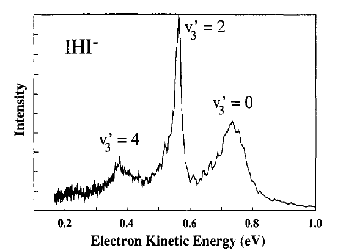
Figure 1.24. Photoelectron spectrum of IHI- → IHI + e- producing the neutral IHI in the v3' = 0, 2, or 4 level of its I···H···I asymmetric stretching mode.
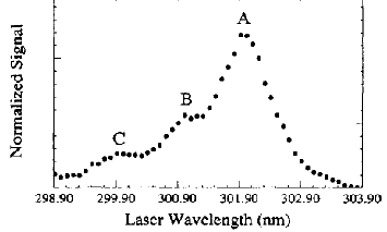 Figure 1.25. Threshold photodetachment spectrum of IHI- → IHI + e- producing the neutral IHI in the v3' = 2 level of its I···H···I asymmetric stretching mode.
The spacings among the v3' = 0, 2, and 4 peaks in Fig. 1.24 are ca. 1400 cm-1; this progression corresponds to the asymmetric I···H···I vibrational mode in the neutral. The spacings among peaks A, B, and C in Fig. 1.25 are ca 100 cm-1 and correspond to the symmetric IHI stretching mode. So, from Fig. 1.24 we can do not see a resolved symmetric stretching progression within the v3' = 2 band (although there may be signs on the left side of this peak). However, in the higher-resolution photodetachment spectrum of Fig. 1.25, the symmetric stretching progression is clear.
Another kind of action spectrum has proven very useful in studying molecular anions arises when one wishes to probe the vibrational spectra of anions using infrared (IR) light. Again, it is essentially impossible to carry out a straightforward IR absorption (or emission) spectrum on a molecular anion sample; the number density of ions and the weak IR oscillator strength do not allow this. However, if one attaches to the molecular anion of interest M- a passive species such as one or more noble gas atoms (e.g., Arn) and subjects the M-···Arn mass-selected ion to IR radiation, one can succeed. In Fig. 1.26 we show an example [[32]] from Professor Mark Johnson's group of an IR spectrum of OH-(H2O)n (n = 1, 2, ... 5) obtained by monitoring for the appearance (this is the action) of OH-(H2O)n ions when mass-selected OH-(H2O)nAr ions are irradiated with IR light. The OH-(H2O)n ions are formed when an IR photon is absorbed by an OH stretching mode in OH-(H2O)nAr and the vibrational energy is converted into the motion of the Ar, thus inducing ejection of the Ar atom. Thus, the action signal, the appearance of OH-(H2O)n, is a direct probe of the absorption of IR energy. Because the action signal involves detecting the mass and quantity of ions, it can be measured with high sensitivity and accuracy.
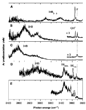
Figure 1.26. Yield of OH-(H2O)n ions from OH-(H2O)nAr as a function of IR photon energy for n = 1 (A) through n = 5 (E).
The features seen in Fig. 1.26 correspond to various vibrations of the OH-(H2O)n complex. For example, F labels a vibrational excitation of a free OH bond (one not involved in hydrogen bonding to the OH- or to other water molecules) and IHB labels a stretching mode for an OH bond that is hydrogen bonded to the OH- ion.
V. Reaction Dynamics Probes
As with spectroscopic probes, there are a variety of different reaction experiments that mass-selected anions are commonly subjected to. In guided-ion beam collision induced dissociation (CID) and collisonal reaction experiments, one accelerates a mass-selected and collimated ion beam to a specificed kinetic energy E (in the laboratory frame) and allows these ions to collide either with an inert gas (in CID) or with a reactant gas (in collisional reaction). The inert or reactant gas usually exists in a collision chamber held at some temperature T, so these gas molecules are moving randomly with a Maxwell-Boltzmann distribution of kinetic energies and with a thermal distribution of internal energies. Upon collisions between the guided-ion beam and the gas in the collision chamber, dissociation or chemical reaction can occur. The products of these events are then subjected to mass analysis and quantitation, again using mass spectrometric means. In carrying out such experiments, one must usually vary the concentration (i.e., the pressure) of the gas molecules to make sure that one is observing single-collision events. One usually does this by extrapolating results to the low-pressure limit.
In a collision between an anion having mass M and an inert or reactive gas molecule of mass m, not all of the laboratory-frame kinetic energy E of the ion is available to induce dissociation or reaction. Only the so-called center-of-mass kinetic energy
ECoM = ½ (mM/(m+M)) vrel2
is available. Here, vrel is the relative velocity with which the ion and the gas molecule collide. If the anion beam's laboratory velocity vLab exceeds the average thermal velocities of the gas molecules, then vrel can be approximated as vLab, and the ECoM can be related to the ion's laboratory kinetic energy E as
ECoM = ½ (mM/(m+M)) vLab2 = (m/(m+M)) E.
This shows that only the fraction m/(m+M) of the laboratory collision energy E is available to induce dissociation or reaction. This fraction can be very low when the ion mass M exceeds that of the collision gas m by a large amount. For this reason, in CID experiments, heavy inert gases such as Xe are often employed.
In Fig. 1.27 we show guided-ion beam measured reaction cross-sections [[33]] for S- anion abstracting a hydrogen atom from H2, methane, or ethane taken from Professor Kent Ervin's laboratory. In these cases, it is the HS- product ions that are detected as a function of the S- ion beam's kinetic energy ECoM.
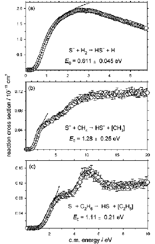
Figure 1.27. Cross-sections for S- abstracting a hydrogen atom from H2 (a), CH4(b) and C2H6(c) as functions of the center-of-mass collision energy in eV.
For the reaction with H2, the threshold was determined to be 59.0 kJ mol-1, which is very close to the endothermicity (59.4 kJ mol-1) of the reaction
S- + H2 → HS- + H.
This suggests that the hydrogen abstraction proceeds with no energy barrier above the endothermicity. In contrast, for reactions with CH4 and C2H6, the thresholds appear at 124 and 107 kJ mol-1, respectively. However, the corresponding endothermicities are 60 and 44 kJ mol-1, suggesting that reaction barriers do exist for these reactions. In addition, the magnitudes of the latter two reactions' cross-sections are much smaller than for the H2 reaction; this is consistent with barriers appearing in the latter but not in the former. Indeed, as shown in Fig. 1.28, barriers are observed in the latter two reactions' potential energy profiles when computed using the methods detailed in Chapter 2. An analogous examination of the energy profile for the reaction with H2 shows no barrier above the reaction endothermicity.
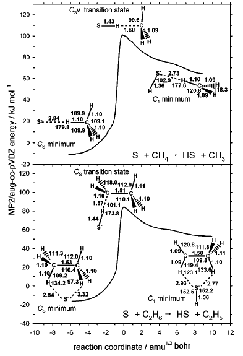
Figure 1.28. Energy as a function of reaction progress along intrinsic reaction paths for S- abstracting a hydrogen atom from methane (top) and ethane (bottom).
To determine the threshold E0 for dissociation or reaction, a model [[34]] for how the cross-section s depends upon collision energy ECoM is employed:
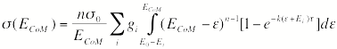 .
.
Here s0 is a parameter related to the maximum of the cross-section and Ei is the energy of the ith internal (vibration-rotation-electronic) state of the reactants whose population is gi. The variable n controls the shape of the energy dependence of s. The time variable t is the average experimental time available for the dissociation or reaction to occur (i.e., how long the ion-molecule collision complex remains in the instrument subject to detection), and k(e+Ei) is the unimolecular rate constant for dissociation of the ion-molecule collision complex having energy equal to Ei +e. If the residence time t is long enough to assure that all collision complexes that are going to dissociate or react have time to do so, the above expression reduces to
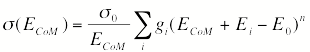 .
.
Clearly, the latter expression shows that s will vanish whenever the available collision energy plus the internal energy of the reactants falls below the threshold E0. So, if one has reasonable knowledge about the populations gi of the reactants' internal states, one can fit this expression to the experimentally observed energy dependence of s to extract E0. However, whenever (e.g, for large molecules) the ion-molecule collision complex survives without fragmenting longer than the experimental residence time t, one cannot use the simplified cross-section expression shown above. In such cases, although the total amount of energy contained within the collision complex may exceed the reaction threshold, it simply takes too long for this energy to end up in the critical reaction coordinate that permits fragmentation to occur.
In Fig. 1.29 we show another example [[35]] of guided-ion beam data from Kent Ervin's laboratory. In this case, an ion complex consisting of HS-···HCN is subjected to collisions with Xe gas and the number and masses of various product ions are determined. Three primary reactions are observed: collision induced dissociation (CID) of the complex to produce HS- (and HCN), proton transfer to yield CN- (and H2S), and formation of HS-···Xe (and HCN). In Fig. 1.30, we see the reaction energy profile computed in ref. 35.
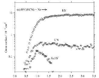
Figure 1.29. Guided-ion beam cross-sections for dissocitation of HS-···HCN complex by Xe atoms as functions of collision energy (eV)
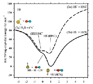
Figure 1.30. Reaction energy profiles for HS-···HCN (solid line) and HS-···(HNC) (dashed line) to yield HS- + HCN (right) and H2S + CN- (left) vs. reaction coordinate.
An interesting feature of the data shown in Fig. 1.29 is that, while the thresholds for production of HS- + HCN and H2S + CN- are nearly identical (ca. 0.4 eV), the maximum magnitudes of the corresponding cross-sections differ by approximately a factor of ten. The reaction energy profiles for forming these two products seen in Fig. 1.30 suggest that the thresholds for forming these two products should indeed be similar. By using the kind of electronic structure tools discussed in Chapter 2, the workers of ref. 35 we able to determine the energies, geometries, and vibrational frequencies of the transition states connecting HS-···HCN to HS- + HCN and to H2S + CN-. They found that the transition state leading to H2S + CN- is very tight (i.e., a compact structure with high-frequency inter-fragment vibrations) while that leading to HS- + HCN is loose. These structural differences in the transition states caused rates to differ by an order of magnitude (i.e., because the transition state's partition function for forming HS- + HCN is larger than that for forming H2S + CN-).
Another instrumental setup that has produced a wealth of data on reactions of molecular anions is referred to as a flow tube. An example of this instrument (used for positive-ion studies in this case) is shown schematically in Fig. 1.31.
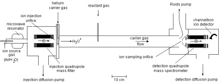
Figure 1.31. Schematic of a flow tube instrument.
In this kind of experiment, ions are typically created (at the left in Fig. 1.31) using an electric discharge within a flowing gas containing precursors of the anions of interest and a carrier gas (He in Fig. 1.31). This discharge creates cations, radicals, and anions, many in excited electronic states that often emit an observable visible glow, so such setups often are called flowing afterglow instruments. Subsequent to creating this ion and radical mixture, a mass-selection device such as the quadrupole mass filter shown in Fig. 1.31 can be used to extract ions of a given charge and q/m ratio and to allow these ions to enter the flow tube region. Such a mass selection step within the flow tube instrument is described as using a selected-ion flow tube or SIFT step. After exiting the mass filter, the selected ions flow, under a carrier gas from left to right through the flow tube. While in this tube, the ions can be subjected to collisions with other gases that can be injected using any of the gas inlet ports as shown in Fig. 1.31.
The anions, carrier gas, and any injected reactant gas flow down the tube at a fixed velocity v (determined by the pressure of the carrier gas). So, the time t it takes for an anion (or reactant or carrier species) to move from the location of an inlet port to the end of the flow tube where it enters the detection region (right of the flow tube in Fig. 1.31) will be related to the distance d separating the inlet port and the detection region by
t = d/v.
So, by injecting reactants at various inlet ports, one can vary d; and by changing the flow rate, one can alter v. Through both of these means, one can alter the time interval t over which the selected anions are in contact with a reactant gas. Of course, the range of flow rates that can be achieved and physical limits on the length of the flow tube place limits on the time t, which, in turn, limits the rates of reactions that can be studied by such flow tube methods.
Assuming that the anions A- and the reactant gas molecules B undergo bimolecular collisions to generate product ions P-
A- + B → P-,
the rate of appearance of P- ions should be determined by the following kinetic equation
d[P-]/dt = k [B] [A-] = - d[A-]/dt
If, as is usually the case, the concentration of the reactant gas greatly exceeds that of the reactant anions, the concentration [B] will remain essentially unchanged (at [B]0) throughout the reaction, so this kinetic expression will reduce to a pseudo- first-order form
d[P-]/dt = k [B]0 [A-] = - d[A-]/dt,
which can be integrated to yield
[A-](t=t) = [A-](t=0) exp(-k[B] t), and
[P-] = [A-](t=o) (1-exp(-k[B] t)).
Here, t = 0 corresponds to the time the anions pass the inlet port at which reactant gas B is injected, and t = t is the time when this collection of gases (ions, neutrals, and carrier gas) exit the flow tube and enter the detection region. Because t is given by d/v, these solutions to the kinetic equations can be written in terms of exp(-k[B]d/v) instead.
So, one carries out a series of such experiments in which the reactant gas molecules B are injected from inlet ports at varying distances from the detector. By then monitoring the concentration of A- ions or of product P- ions arriving at the detector, one can, for example, plot ln[A-] vs. the distance d to extract the pseudo first-order rate constant k[B]. An example of such a plot is shown in Fig. 1.32 from an experiment in Professor Veronica Bierbaum's lab [[36]] where the reaction of the isoprene anion H2C=CH-(CH2)2- with D2O to exchange one, two or three D atoms for H atoms has been studied. Knowing the flow velocity v and the concentration of D2O, these workers could also determine the rate constants for these reactions.
Figure 1.32. Percent of allyl anions that have undergone one (d1) through three (d3) deuterium-for-hydrogen atom exchanges as a function of distance along the flow tube.
Another example from this same lab [[37]] in a study of F- anions reacting with H3C-OOH produces the data shown in Fig. 1.33 in which the flow tube distance variable d has already been converted to time using the known flow velocity.
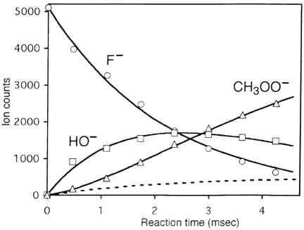
Figure 1.32. Concentrations of F- reactant and OH-, and CH3-OO- product ions as functions of time.
An interesting lesson learned in this study is that the H3COO- anion is not formed only by proton abstraction from the O-H unit
F- + H3C-OO-H → FH + H3C-OO-.
Instead, a proton can be lost from the methyl group
F- + H3C-OOH →-H2C-OOH + FH
after which the -H2C-OOH anion decomposes to produce OH- and formaldehyde
-H2C-OOH → OH- + H2C=O.
The OH- can then go on to react with another H3C-OOH to generate the H3C-OO- anion in another route
OH- + H3C-OOH → H2O + H3C-OO-.
The amount of H3C-OO- produced by direct proton abstraction is shown by the dashed line in Fig. 1.32; the total amount is shown in the solid line.
Professor Paul Kebarle carries out a different kind of experiment using mass spectrometric tools. In particular, he studies ion reactions under equilibrium conditions, and, by determining the temperature dependence of various equilibrium constants, he determines reaction DH and DS vallues. An example of one of his studies [[38]] of the (OH)2PO2- anions being sequentially hydrated
(OH)2PO2-(H2O)n-1 + H2O → (OH)2PO2-(H2O)n
produced the data shown in Fig. 1.33.
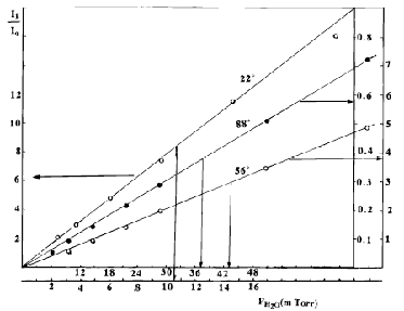
Figure 1.33 Observed intensity ratio for (OH)2PO2- ions with one (I1) and zero (I0) water molecules attached as a function of water pressure at three temperatures (22, 56, and 88 C).
The equilibrium constant K0,1 for the equilibrium
(OH)2PO2-(H2O)n-1 + H2O ⇔ (OH)2PO2-(H2O)n
is obtained as the slope of the I1/I0 plot vs. P(H2O). When these equilibrium constants, determined at various temperatures are then plotted vs. 1/T to form a van 't Hoff plot, Fig. 1.34 was obtained.
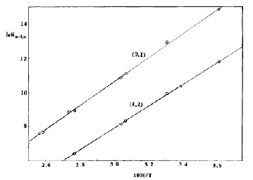
Figure 1.34. Van 't Hoff plot of K0,1 and K1,2 vs. 1/T for sequential hydration of (OH)2PO2-
From the slopes and intercepts of these two plots, the Kebarle group obtained DH0,1 = -14.0, DH1,2 = - 12.3 kcal mol-1 and DS0,1 = -21.0, DS1,2 = -20.8 cal mol-1 K-1. Using this kind of equilibrium measurement, the Kebarle group has been able to determine sequential hydration energies (and energies for binding many other ligands) for a wide variety of anions and cations.
This concludes the discussion of how anions are made, controlled, and studied in the laboratory. As I said earlier, because my background lies in theoretical chemistry, I am not able to offer as much insight into such matters as a first-rate experimental chemist who studies molecular anions. For this reason, I encourage the reader to go to the web sites of some of the experimental chemists I mention througout this text to learn in more detail how the experiments are carried out and about their limitations and sources of error. Now, let us turn our attention to some of the challenges that molecular anions pose to their theoretical study.
Chapter 2. Anions Also Present Special Challenges to Theoretical Study
There are several sources that one can access to read about how the theoretical study of anions has evolved over the past few decades. These include reviews by: Boldyrev and Gutsev [[39]], Baker, Nobes, and Radom [[40]], Jordan [[41]], Simons and Jordan [[42]], Kalcher and Sax [[43]], Kalcher [[44]] and Berry [[45]], as well as classic earlier overviews by Massey [[46]] and Branscomb [[47]], and a book [[48]] edited by Professor Josef Kalcher. Later in this text, other review articles relating to particular families of anions are also cited.
The reader may expect this Chapter will conclude with specific recommendations about the theoretical tools that are optimal for studying anions and computing EAs. Unfortunately, this is not going to be possible although there are certain aspects (e.g., the use of special diffuse basis sets and the need to treat what is called electron correlation) that are common to any good approach for theoretically studying anions. The fact is there are several reliable and accurate theoretical approaches that can be used; some are better in certain circumstances and others are better in others. Moreover, the computational effort and degree of accuracy involved in various methods varies greatly from method to method, with the most accurate approaches almost always having the highest computational demand. In addition, this demand scales in a highly non-linear (e.g., as the third or higher power of the number of electrons) manner with the size of the molecule. It is therefore not always practical to invoke the most accurate calculation, so one is often faced with balancing computational effort against needed accuracy. For such reasons, it is necessary to explain the strengths and weaknesses of several different methods so the reader will understand and thus be optimally positioned to apply the most appropriate methods in cases of her or his interest.
Before discussing many of the theoretical methods available for calculating EAs and studying the structures, energies, reactivities, and spectroscopic behavior of anions, I want to first reiterate the magnitude of the difficulty inherent in these tasks by considering how small a percent of the total electronic energy the EA is. Let us begin with the simplest case and the situation in which the task appears the most straightforward. For the anion containing the fewest electrons H-, the EA is 0.75 eV whereas the total electronic energy is –14.35 eV (i.e., the sum of the EA and the ionization energy of H). So, for H, the EA is 5.2 % of the total energy. Therefore, if one is able to compute total electronic energies of H and H‑ accurate to a few percent, computation of this EA to within an accuracy of say 30% appears to be quite feasible.
However, for atoms and molecules containing more electrons, the situation is much worse because the total electronic energy grows rapidly with the number of electrons, whereas the EAs of most atoms and molecules remain in the 0.01- 4 eV range.
So, if one has available a tool that promises to compute electronic energies to say 1%, one soon (i.e., for some reasonable size molecule) finds that the full magnitude of the EA is less than this percent of the total electronic energy.
To further illustrate, let us consider the EA of a carbon atom which has been measured by examining the C-(4S3/2) → C(3P0) photodetachment threshold to be 1.262119 ± 0.000020 eV. The total electronic energy of the C atom is –1030.080 eV (obtained by adding the C → C+, C+→ C2+ , C2+→ C3+ , C3+→ C4+, C4+→ C5+, and C5+→ C6+ ionization energies). The total energy is a negative quantity because the ground-state energy of C is defined (as is the case for all atoms and molecules) relative to a reference in which the zero of energy corresponds to the bare nuclei and bare electrons all infinitely far from one another and all having no kinetic energy. To compute the EA of C even to an accuracy of 0.1 eV requires either
- that one compute the total electronic energies of both C and C-to this accuracy (which is only 9.7 x10⁻³% of the total energy) or
- one rely on cancellation of systematic errors when these two energies are subtracted to obtain the EA.
In any event, as we discussed earlier in this text, the evaluation of EAs is complicated by the fact that total electronic state energies are extensive quantities but EAs are intensive quantities as was noted earlier in this text.
Not surprisingly, much of the total energy of a carbon atom derives from the energies of the two 1s electrons (as reflected in the fifth and sixth ionization energies being 392.077 and 489.981 eV, respectively), To the extent that the 1s inner-shell electrons are unaffected by adding an electron to C to form C-, errors made in computing their total energy contributions should cancel when EA is calculated. As most chemists know well, inner-shell orbitals are indeed little affected by changes made to the valence-orbital occupancies. However, the inner-shell orbitals are altered to some extent, even if only to a small degree. Thus, if one is faced with the challenge of computing EAs to high accuracy, one cannot ignore changes in the core orbitals' energies. However, one often relies on the approximate cancellation of the energies of the inner-shell electrons and computes EAs by focusing much of the computational detail and effort on the dynamics of the valence-level electrons. This approach is usually capable of yielding EAs accurate to ca. 30% if one handles what is called the correlation energy of the valence-level electrons using methods that we detail later.
Another issue to be aware of is the magnitude of the electron-electron Coulomb interaction in comparison with the total energies. This is important because it is precisely these contributions to the total energies that essentially all quantum chemistry tools have difficulty treating to high accuracy, and it is these energies that render the Schrödinger equation not analytically (or even numerically to high precision) soluble for atoms and molecules. Again using the C/C- example, we note that the difference between the fifth and sixth ionization energies of the C atom is ca. 97 eV. This difference offers an estimate of the Coulomb repulsion between the two 1s electrons. Clearly, because these two electrons reside in close proximity to one another on average, their repulsion is quite large. In contrast, the difference between the first and second ionization energies is ca. 13 eV, which gives an estimate of the Coulomb repulsion between two electrons in two orthogonal 2p orbitals of C (e.g., 2px and 2py). Even this repulsion energy is large when compared to the accuracy (i.e., ca. 0.1 eV) to which we usually aspire to compute atomic and molecular EAs.
The relevance of these observations about the sizes of Coulomb interactions is that essentially all quantum chemistry methods begin with a so-called mean-field description of these interactions (e.g., as in the Hartree-Fock method discussed later in thi Chapter). That is, the interactions are approximated in terms of a Coulomb integral
Ji,j = ∫ |fi(r)|2 e2/|r-r'| |fj(r')|2 dr dr',
where |fi(r)|2 and |fj(r')|2 give the mean-field estimates of the spatial probability densities for finding an electron in orbital fi at location r and another electron in fj at location r', respectively. This estimate of the average Coulomb interaction between the pair of electrons is not fully correct because it ignores correlations in the electrons' motions. That is, it assumes that the probability density for finding one electron at r does not depend on where the other electron is located. It turns out that such uncorrelated estimates of Coulomb interactions between pairs of electrons are accurate to 5-10 %. However, for the two 2p orbitals of C discussed above, a 5-10 % error in the interaction energy of 13 eV is still too large an error to tolerate if one is attempting to compute the EA of C to within 0.1 eV. For such reasons, one is forced to use theoretical descriptions of the electronic structures of the neutral and anion that more adequately describe the correlated movements of at least the valence-level orbitals (then assuming that systematic errors in the energies of the inner-shell orbitals cancel). Several approaches to treating inter-electron correlations are described later in this Chapter.
Having given insight into the fundamental difficulties behind accurate evaluation of atomic or molecular EAs (e.g., EAs are intensive and small fractions of total energies, and electrons undergo correlated not mean-field motions), let us now move on to discuss the variety of tools that can be applied to this challenging task.
I. Special Atomic Basis Sets Must be Used
Because of the diffuse character of the electron densities of anions, one must employ atomic orbital (AO) basis sets that decay slowly with radial distance r. As noted earlier, because electron binding energies are, by nature, small quantities, one must compute EAs with high absolute accuracy to achieve acceptable percent errors. The latter fact requires that the AO basis set be flexible enough to describe accurately the spatial distributions of the electrons as well as their so-called dynamical correlation (we discuss this later). That is, the quality of the basis influences both our ability to describe the radial and angular shapes of the orbitals that contain the electrons as well as our ability to treat the correlated motions of the electrons.
Let us now briefly review what constitutes the kinds of AO bases that are most commonly used for such studies. The basis orbitals commonly used to express the molecular orbitals (MOs) fj as linear combinations of AOs cm via the linear combination of AOs to form MOs (LCAO-MO) process fall into two primary classes:
- Slater-type orbitals (STOs) have the following angular and radial form
cn,l,m (r,q,f) = Nn,l,m,z Yl,m (q,f) rn-1 exp(-zr)
and are characterized by quantum numbers n, l, and m and exponents (which characterize the radial 'size' ) z. The symbol Nn,l,m,z denotes the normalization constant.
- Cartesian Gaussian-type orbitals (GTOs) have the following angular and radial form
ca,b,c (r,q,f) = N'a,b,c,a xa yb zc exp(-ar2),
and are characterized by quantum numbers a, b, and c, which detail the angular shape and direction of the orbital, and exponents a which govern the radial 'size'.
For both types of AOs, the coordinates r, q, and f refer to the position of the electron relative to a set of axes attached to the center on which the basis orbital is located. It is most common to locate such orbitals on the atomic nuclei, but, at times, additional so-called floating AOs are placed elsewhere. For example, when describing the binding of an electron to the NH4+ cation discussed earlier, it would be appropriate to center diffuse s-type basis functions designed to treat this species' Rydberg orbital on the nitrogen nucleus. When studying an electron solvated within a cavity formed by four tetrahedrally placed H2O molecules whose dipoles are oriented inward, one most likely would place floating s- and p- type AOs at the center of the tetrahedral cavity rather than on any of the O or H nuclei of the surrounding water molecules. Of course, if any basis were mathematically complete, it would not matter where the functions were located. However, it is essentially never possible to utilize a complete basis or one that approaches completeness, so one is usually forced to choose where to place the AOs based upon knowledge or intuition about where the attractive potential is likely to accumulate electron density.
The two families of basis AOs mentioned above have their own strengths and weaknesses. Slater-type orbitals are similar to Hydrogenic orbitals in the regions close to the nuclei. Specifically, they have a non-zero slope near the nucleus on which they are located (i.e., d/dr(exp(-zr))r=0 = -z) and the more radially compact the STO, the larger is this slope. In contrast, GTOs, have zero slope near r=0 because d/dr(exp(-ar2))r=0 = 0. We say that STOs display a cusp at r = 0 that is characteristic of the Hydrogenic solutions, whereas GTOs do not. This characteristic favors STOs over GTOs because we know that the correct solutions to the Schrödinger equation have such cusps at each nucleus of a molecule (because near a nucleus the –Ze2/r potential is dominant).
Although STOs have the proper 'cusp' behavior near nuclei, they are used primarily for atomic and linear-molecule calculations because the multi-center integrals that arise in polyatomic-molecule calculations (we will discuss them later) cannot efficiently be evaluated when STOs are employed as basis AOs. In contrast, such integrals can routinely be computed when GTOs are used. This fundamental advantage of GTOs has lead to the dominance of these functions in molecular quantum chemistry.
To overcome the primary weakness of GTO functions (i.e., their radial derivatives vanish at the nucleus), it is common to combine two, three, or more GTOs, with combination coefficients that are fixed and not treated as LCAO parameters, into new functions called contracted GTOs or CGTOs. Typically, a series of tight, medium, and loose GTOs (i.e., functions with large, intermediate, and small exponents a) are multiplied by contraction coefficients and summed to produce a CGTO that approximates the proper 'cusp' at the nuclear center. However, it is not possible to correctly produce a cusp by combining any number of Gaussian functions because every Gaussian has a zero slope at r = 0 as illustrated in Fig. 2.1.
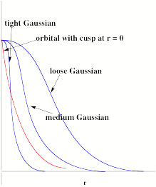
Figure 2.1. Plots of a tight, medium and loose Gaussian radial function showing the zero slope that all Gaussians have at r = 0 as well as the function the contraction of the Gaussians attempts to approximate.
Although most calculations on molecules are now performed using Gaussian orbitals, it should be noted that other basis sets can be used as long as they span enough of the regions of space (radial and angular) where significant electron density resides. In fact, it is possible to use plane wave orbitals [[49]] of the form
c (r,q,f) = N exp[i(kx r sinq cosf + ky r sinq sinf + kz r cosq)],
where N is a normalization constant and kx , ky , and kz are quantum numbers detailing the momenta of the orbital along the x, y, and z Cartesian directions. The advantage to using such simple orbitals is that the integrals one must perform are much easier to handle with such functions; the disadvantage is that one must use many such functions to accurately describe sharply peaked charge distributions of, for example, inner shell core orbitals as well as the slowly-varying diffuse orbitals characteristic of anions' valence regions.
Much effort has been devoted to developing sets of STO or GTO basis orbitals for main-group elements and the lighter transition metals. This ongoing effort is aimed at providing standard basis set libraries which:
- Yield predictable chemical accuracy in the resultant energies (for the ground and excited and ionized states).
- Are computationally cost effective to use in practical calculations.
- Are relatively transferable so that a given atom's basis is flexible enough to be used for that atom in various bonding environments.
Each such basis set has several components designed to handle various aspects of the electronic structure issue. In the following sub-sections, we briefly describe these components.
A. The Fundamental Core and Valence Basis
Within this category, the following choices are common (we illustrate these choices for Gaussian type orbitals because they are the most commonly used):
- A minimal basis in which the number of CGTO orbitals is equal to the number of core and valence atomic orbitals in the atom. For example, for a carbon atom, one would use one tight s-type CGTO, one looser s-type CGTO and a set of three (i.e., x, y, and z) looser p-type CGTOs.
- A double-zeta (DZ) basis in which one uses twice as many CGTOs as there are core and valence atomic orbitals (e.g., two tight s, two looser s, and two sets of three looser p CGTOs for carbon). The use of more basis functions is motivated by a desire to provide additional variational flexibility so the LCAO process can generate molecular orbitals of variable diffuseness as the local electronegativity of the atom varies. For example, the 2p molecular orbital in a neutral carbon atom does not have the same radial extent as the lone pair 2p orbital in the H3C‑anion, so one needs to have a basis set that can describe either 2p orbital. In the DZ basis, the neutral carbon's 2p orbital would have a larger LCAO-MO coefficient multiplying the tighter p-type basis function; the CH3-lone pair orbital would have a larger coefficient multiplying the looser basis function.
- A triple-zeta (TZ) basis in which three times as many CGTOs are used as the number of core and valence atomic orbitals (extensions of this sequence of NZ bases to quadruple-zeta and higher-zeta bases also exist).
Optimization of the orbital exponents (z's or a's) and the GTO-to-CGTO contraction coefficients for the kind of bases described above has undergone explosive growth in recent years. The theory group at the Pacific Northwest National Labs (PNNL) offer a world wide web site from which one can find (and even download in a form prepared for input to any of several commonly used electronic structure codes) a wide variety of Gaussian atomic basis sets.
B. Polarization Functions
One usually enhances any core and valence functions by adding a set of so-called polarization functions. These are functions of one higher angular momentum than appears in the atom's valence orbital space (e.g, d-functions for C, N, and O and p-functions for H), but they have exponents (z or a) that cause their radial sizes to be similar to the sizes of the valence orbitals (i.e., the polarization p orbitals of the H atom are similar in size to the 1s orbital and the polarization d orbitals of C are similar in size to the 2s and 2p orbitals). Thus, polarization functions are not orbitals that describe the atom's valence orbital with one higher l-value; such higher-l valence orbitals would be radially more diffuse. For example, a carbon atom's 3d orbital in, for example, its 1s2 2s2 2p1 3d1 configuration is quite different in radial character from the polarization d-orbital, which has a radial extent similar to the 2p orbital.
One primary purpose of polarization functions is to give additional angular flexibility to the LCAO process in forming bonding molecular orbitals between pairs of valence atomic orbitals. This is illustrated in Fig. 2.2 where polarization dp orbitals are seen to contribute to formation of the bonding p orbital of a carbonyl group by allowing polarization of the carbon atom's pp orbital toward the right and of the oxygen atom's pp orbital toward the left.
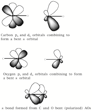
Figure 2.2. Illustrations of the use of polarization functions of p symmetry in CO.
Polarization functions are essential in strained ring compounds such as cyclopropane and cyclopropene because they provide the angular flexibility needed to direct the electron density into regions between bonded atoms. It is just not possible to hybridize the carbon 2s and 2p orbitals to construct bonds that have ca. 60 bond angles as in the above cyclic compounds.
Polarization functions are not only important for allowing charge density to flow into regions between atoms and to thus form directed bonds. It turns out that polarization functions are also important for describing the correlated motions of electrons (this is described in greater detail later in this Chapter), especially their angular correlations. Simply put, electrons avoid one another because they have identical charges. They can do this by moving in different radial regions; that is, one electron can be at small-r when another is at large-r. Alternatively, they can undergo angular correlations; one electron can be on the left while another is on the right. For treating such angular correlations, basis functions having angular momentum quantum numbers higher than those of the valence orbitals are useful to include. In fact, to achieve highly accurate descriptions of angular correlation, one must employ basis functions having quite high L-values. Substantial effort has been devoted to analyzing the L-dependence of the electronic energy so that results obtained from bases obtaining modest L-values can be extrapolated to high-L thus obviating the need to perform calculations with the high-L basis. We will have more to say about such complete-basis extrapolation strategies later.
C. Diffuse Functions
When dealing with anions or Rydberg species, one must further augment the AO basis set by adding so-called diffuse basis orbitals. The valence and polarization functions described above may not provide enough radial flexibility to adequately describe either of these cases. Once again, the PNNL web site database offers a good source for obtaining diffuse functions appropriate to a variety of atoms but not for situations in which very weakly bound anions (e.g., having EAs of 0.1 eV or less) occur.
These tabulated diffuse functions are appropriate if the anion under study has its
excess electron in a valence-type orbital (e.g., as in F-, OH-, carboxylates, MgF42-, etc.). However, if the excess electron resides in a Rydberg orbital, in an orbital
centered on the positive site of a zwitterion species (we will discuss these cases
in Chapter 4), or in a so-called dipole-bound orbital (we will also treat them in
Chapter 4), one must add to the bases containing valence, polarization, and conventional
diffuse functions yet another set of functions that are extra diffuse. The exponents of these extra diffuse basis sets should be small enough to describe
the diffuse charge distribution of the excess electron. In dipole-bound anions, not
only s but also p and sometimes d symmetry functions are required to describe a dipole-bound
orbital localized on the positive side of the molecular dipole. For example, in the
NCH- dipole-bound anion, the extra diffuse functions would likely be centered on the H
atom because this nucleus is near the positive end of HCN's dipole as shown in Fig.
2.3.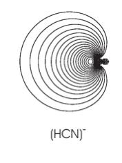
Figure 2.3. Orbital holding the excess electron in HCN-; the hydrogen nucleus is on the left side of the molecular framework which can barely be seen because of the large size of the orbital.
It would be essentially impossible to describe such a diffuse orbital using conventional AO basis sets even when conventional diffuse functions are included.
Moreover, the extra-diffuse set of AOs needs to be flexible enough to describe dispersion stabilization between the excess electron and the electrons of the neutral species. Dispersion is also an electron correlation effect, so the remarks made in the preceeding subsection about using basis functions of higher L-values also apply to it. In the NCH- example discussed above, the dispersion interaction we refer to is that between the electron in the large, diffuse, highly polarizable dipole-bound orbital shown in Fig. 2.3 and the fourteen electrons of the HCN molecule. We note that the kind of extra diffuse basis sets discussed here have been developed [[50]] by the author and Professors Maciej Gutowski and Piotr Skurski and are currently experiencing wide use in the electronic structure community.
D. Basis Notations
It has become common to describe valence, polarization, and (conventional) diffuse AO basis sets using one of several short hand notations. The various notations derive from the rich history of the several research groups that developed these now widely used basis sets. Rather than review this history, we will simply summarize the notations that are most commonly used. First, it is common in all of the basis sets we will discuss to treat the core and valence atomic orbitals (e.g., for carbon the 1s orbital is a core orbital and the 2s and 2p are valence; for transition metals such as Ti, the 3d and 4s orbitals constitute the valence and the 1s, 2s, 2p, 3s, and 3p are the core) differently. In particular, a more flexible set of contracted orbitals is usually employed for the valence orbitals because it is the valence orbitals that change most (i.e., in their radial extent) depending on what other atoms are involved in the bonding.
The AO basis sets developed largely by Thom Dunning and co-workers use notation of the following form: aug-cc-pVTZ or cc-pVQZ or pVDZ. The VDZ, VTZ, VQZ or V5Z component of the notation is used to specify at what level (double-zeta DZ, triple-zeta TZ, quadruple zeta QZ, or quintuple zeta 5Z) the valence (V) AOs are described. Nothing is said about the core orbitals because each of them is described by a single contracted Gaussian type basis orbital. The term cc is used to specify that the orbital exponents and contraction coefficients in each of the contracted AOs were determined by requiring the atomic energies (usually of all term symbols arising from the conventional lowest-energy electronic configuration), when computed using a correlated rather than Hartree-Fock method, agree to within some tolerance with experimental data. If cc is missing from the notation, the AO exponents and contraction coefficients were determined to make the Hartree-Fock atomic state energies agree with experiment to some precision. The notation p is used to specify that polarization basis orbitals have been included in the basis (if the p is absent, no polarization functions have been added). However, the number and kind of polarization functions differs depending on what level (i.e., VDZ through V5Z) the valence orbitals are treated. At the VDZ level, only one set of d polarization functions is added; at the VTZ, two sets of d and one set of (7) f polarization functions are included. At the VTZ level, three d, two f, and one g set of polarization functions are present, and at the V5Z, four d, three f, two g and one h sets of polarization functions are included. The notation aug is used to specify that (conventional) diffuse basis functions have been added to augment the basis, but again the number and kind depend on how the valence basis is described. At the pVDZ level, one s, one p, and one d diffuse function appear; at pVTZ a diffuse f function also is present; at pVQZ a diffuse g set is also added; and at pV5Z a diffuse h set is present.
For example, a carbon atom basis of aug-cc-p-VTZ quality has a single 1s contracted function, three s-type (i.e., of three distinct radial extent because the valence basis is of triple-zeta quality) valence functions, three sets (i.e., x, y, z) of p-type valence functions of various radial size, two sets (xy, xy, yz, x2-y2, z2) of d-type polarization functions (having radial size similar to the valence s and p functions), one set (containing seven) of f-type polarization functions, a more diffuse s and sets (x, y, z) of more diffuse p, d, and f functions. This basis thus contains a total of 46 contracted AOs. An aug-cc-p-VDZ basis would contain 23 AOs, an aug-cc-p-VQZ basis 80, and an aug-cc-p-V5Z basis 127 AOs. A full listing of the aug-cc-p-V5Z basis is shown below with the left column telling the kind of CGTO (i.e., s, p, d, etc.) as well as the Gaussian orbital exponents (aJ) of each primitive Gaussian and the right column giving the contraction coefficient telling how to combine the primitive Gaussians to form the contracted Gaussian AO.
CARBON, Aug-cc-pV5Z: (127 basis functions, 209 primitive functions)
Standard basis: Aug-CC-pV5Z (5D, 7F)
Basis set in the form of general basis input:
1 0
S   10 1.00
0.9677000000D+05  0.2500000000D-04
0.1450000000D+05  0.1900000000D-03
0.3300000000D+04  0.1000000000D-02
0.9358000000D+03  0.4183000000D-02
0.3062000000D+03  0.1485900000D-01
0.1113000000D+03  0.4530100000D-01
0.4390000000D+02  0.1165040000D+00
0.1840000000D+02  0.2402490000D+00
0.8054000000D+01  0.3587990000D+00
0.3637000000D+01  0.2939410000D+00
S   10 1.00
0.9677000000D+05 -0.5000000000D-05
0.1450000000D+05 -0.4100000000D-04
0.3300000000D+04 -0.2130000000D-03
0.9358000000D+03 -0.8970000000D-03
0.3062000000D+03 -0.3187000000D-02
0.1113000000D+03 -0.9961000000D-02
0.4390000000D+02 -0.2637500000D-01
0.1840000000D+02 -0.6000100000D-01
0.8054000000D+01 -0.1068250000D+00
0.3637000000D+01 -0.1441660000D+00
S    1 1.00
0.1656000000D+01  0.1000000000D+01
S    1 1.00
0.6333000000D+00  0.1000000000D+01
S    1 1.00
0.2545000000D+00  0.1000000000D+01
S    1 1.00
0.1019000000D+00  0.1000000000D+01
P    4 1.00
0.1018000000D+03  0.8910000000D-03
0.2404000000D+02  0.6976000000D-02
0.7571000000D+01  0.3166900000D-01
0.2732000000D+01  0.1040060000D+00
P    1 1.00
0.1085000000D+01  0.1000000000D+01
P    1 1.00
0.4496000000D+00  0.1000000000D+01
P    1 1.00
0.1876000000D+00  0.1000000000D+01
P    1 1.00
0.7606000000D-01  0.1000000000D+01
D    1 1.00
0.3134000000D+01  0.1000000000D+01
D    1 1.00
0.1233000000D+01  0.1000000000D+01
D    1 1.00
0.4850000000D+00  0.1000000000D+01
D    1 1.00
0.1910000000D+00  0.1000000000D+01
F    1 1.00
0.2006000000D+01  0.1000000000D+01
F    1 1.00
0.8380000000D+00  0.1000000000D+01
F    1 1.00
0.3500000000D+00  0.1000000000D+01
G    1 1.00
0.1753000000D+01  0.1000000000D+01
G    1 1.00
0.6780000000D+00  0.1000000000D+01
H    1 1.00
0.1259000000D+01  0.1000000000D+01
S    1 1.00
0.3940000000D-01  0.1000000000D+01
P    1 1.00
0.2720000000D-01  0.1000000000D+01
D    1 1.00
0.7010000000D-01  0.1000000000D+01
F    1 1.00
0.1380000000D+00  0.1000000000D+01
G    1 1.00
0.3190000000D+00  0.1000000000D+01
H    1 1.00
0.5860000000D+00  0.1000000000D+01
****

127 basis functions      209 primitive gaussians
The AO basis sets developed largely by the late Professor John Pople and co-workers use a different notation to specify essentially the same information. For example, they use notation of the form 6-31+G** or 3-21G*, 6-311+G*, or 6-31++G. The 3- or 6- component of the notation is used to specify that the core orbitals are each described in terms of a single contracted Gaussian orbital having 3 or 6 terms in its contraction. The –21 or –31 is used to specify that there are two valence basis functions of each type (i.e., the valence basis is of double-zeta quality), one being a contraction of 2 or 3 Gaussian orbitals and the other (the more diffuse of the two) being a contraction of a single Gaussian orbital. When –311 is used, it specifies that the valence orbitals are treated at the triple-zeta level with the tightest contracted function being a combination of 3 Gaussian orbitals and the two looser functions being a single Gaussian function. The * symbol is used to specify that polarization functions have been included on the atoms other than hydrogen; the ** specifies that polarization functions are included on all atoms, including the hydrogen atoms. Finally, the + is used to denote that a single set of (conventional) diffuse valence basis AOs have been included; ++ means that two such sets of diffuse valence basis AOs are present.
Finally, we should say that no common notation exists to specify that extra diffuse basis AOs such as those needed for very weakly bound anions are included. One must simply state this explicitly when detailing the AO basis sets that are employed. It is useful to point out that the kind of extra diffuse basis sets that have been designed for such purposes were constructed by taking each conventional diffuse valence AO and adding a series of successively more diffuse orbitals of identical angular character but with orbital exponents aJ that are related in an even tempered manner to the exponent aO of the conventional diffuse AO. For example, to add three extra diffuse p-type AOs to a carbon atom whose conventional diffuse p-type AO has an exponent of 0.25, we would add p-functions with exponents 0.25/3, 0.25/9 and 0.25/27 (i.e., with an even tempering scale factor of 1/3).
E. Computational Cost Depends on the Basis Size
It is essential to be aware of the total number of AO basis functions used in a calculation because the computational cost (i.e., CPU time) and data storage (in main memory or on disk) involved in various calculations depends in a highly non-linear manner on the basis size which I will denote M. The non-linear scaling arises primarily from two sources:
- In essentially all calculations of electronic energies and wave functions, certain integrals involving products of two or four Gaussian AOs also involving components of the Hamiltonian operator (i.e., the kinetic energy operator, the electron-nuclei Coulomb potential, or the electron-electron Coulomb potential) need to be computed. The number of such integrals is proportional to the square or the fourth power of the number of AOs, respectively. This results in an M4scaling in the CPU time needed for the evaluation and an M4scaling for the data storage.
- To compute the electronic energy and wave function, one ends up either (a) having to solve for an eigenvalue of a large (sparse) matrix whose dimension varies at least linearly (more likely at least quadratically) with the basis size M or (b) having to sum a number of terms whose number varies as M4or higher. The former case arises in Hartree-Fock (HF) and configuration interaction (CI) calculations and the latter in Møller-Plesset perturbation theory (MPPT) calculations, both of which we discuss later. To solve for a single eigenvalue of a matrix (A) of dimension D requires CPU time proportional to D2because one must compute elements of a vector v equal to the product of the matrix A with another (so-called trial) vector u: vJ = SK AJ,K uK which clearly involves M2 operations. The dimension of the HF Hamiltonian matrix is M, so the CPU time needed to evaluate a single HF molecular orbital and its energy will scale as M2. Because the dimension D of the CI Hamiltonian matrix most likely scales as M2 or higher, the CPU time will vary as M4 or more strongly in CI calculations.
Although we illustrate the strong dependence of CPU time and data storage on the size of the AO basis for only three (HF, CI and MPPT) methods, suffice it to say that the cost of all electronic structure methods can rapidly get out of hand if the AO basis grows too large. For example, an aug-cc-p-VDZ calculation on buckyball C60 would involve 23 contracted Gaussian orbitals per carbon atom or 1380 total AOs. The number of so-called two-electron integrals (we define these later in this Chapter) is M4/8; for this basis there would be 4.5 x10¹¹ such integrals that need to be calculated and (perhaps) stored. For aug-cc-p-VTZ or aug-cc-p-VQZ bases, the total number of AOs would be 2760 or 4800, respectively, and the number of two-electron integrals would be 7.3 x10¹² or 6.6 x10¹³. It would thus appear that, with a modern computer capable of carrying out ca. 109 CPU operations per second (and knowing that each two-electron integral requires several floating-point arithmetic operations to evaluate) that calculations on C60 using any of these bases would be feasible in a few thousand to a million seconds. However if a calculation whose CPU cost scales as M5 were to be employed, these three example calculations would require 1380-4800 times as much effort, which may prove prohibitive even with a 109 operations-per-second computer. It is therefore very important to use bases that are adequate to the task at hand but not unnecessarily large and to anticipate the CPU and storage needs that will arise as a basis is expanded to include additional functions.
II. The Hartree-Fock SCF Process is Usually the Starting Point
Once one has specified an AO basis for each atom in the molecule or anion, the LCAO-MO procedure can be used to determine the Ci,m coefficients that describe the occupied and virtual orbitals. It is important to keep in mind that the basis AOs are not themselves the SCF orbitals of the isolated atoms; even the SCF orbitals are combinations (with atomic values for the Ci,m coefficients) of the basis functions. The LCAO-MO-SCF process itself determines the magnitudes and signs of the Ci,m coefficients, and alternations in the signs of these coefficients allow radial nodes to form.
Because the full electronic Hamiltonian
H = Sj {- h2/2m ∇2j - Ze2/rj} + 1/2 Sj,k e2/|rj-rk|
is invariant under the operation Pi,j in which any pair of electrons have their labels (i, j) permuted, we say that H commutes with the permutation operator Pi,j. This fact implies that any solution Y to HY = EY must also be an eigenfunction of Pi,j As a result of H commuting with electron permutation operators, the eigenfunctions Y must either be odd or even under the application of any such permutation. Because electrons are Fermions, their Y functions must be odd under such permutations.
The simple spin-orbital product function
Y = Pk=1,N fk,
which is what one imagines when one specifies, for example, that carbon is in its 1sa 1sb 2sa 2sb 2pxa 2pya configuration, does not have the correct permutational symmetry. Likewise, the Be atom spin-orbital product wave function
Y = 1sa(1) 1sb(2) 2sa(3) 2sb(4)
is not odd under the interchange of the labels of electrons' 3 and 4 (or of any pair of electrons); instead one obtains 1sa(1) 1sb(2) 2sa(4) 2sb(3) when the permutation is carried out. However, such products of spin-orbitals (i.e., orbitals multiplied by a or b spin functions) can be made into properly antisymmetric functions by forming the determinant of an NxN matrix whose row index K labels the spin orbital and whose column index J labels the electrons. For example, the making Be atom function 1sa(1) 1sb(2) 2sa(3) 2sb(4) antisymmetric produces the 4x4 matrix whose determinant is shown below
| 1sα(1) | 1sα(2) | 1sα(3) | 1sα(4) |
| 1sβ(1) | 1sβ(2) | 1sβ(3) | 1sβ(4) |
| 2sα(1) | 2sα(2) | 2sα(3) | 2sα(4) |
| 2sβ(1) | 2sβ(2) | 2sβ(3) | 2sβ(4) |
Clearly, if one were to interchange any columns of this determinant, one changes the sign of the function. Moreover, if a determinant contains two or more rows that are identical (i.e., if one attempts to form such a function having two or more spin-orbitals equal), it vanishes. This is how such antisymmetric wave functions embody the Pauli exclusion principle.
A convenient way to write such a determinant is as follows:
SP (-1)p fP1 (1) fP2(2) ... fPN(N),
where the sum is over all N! permutations of the N spin-orbitals and the notation (-1)p means that a (–1) is affixed to any permutation that involves an odd number of pairwise interchanges of spin-orbitals and a +1 sign is given to any that involves an even number. To properly normalize such a determinental wave function, one must multiply it by (N!)-1/2. So, the final result is that wave functions of the form
Y = (N!)-1/2 SP (-1)p fP1 (1) fP2(2) ... fPN(N)
have the proper permutational antisymmetry.
If one uses a single-determinental wave function to form the expectation value of the Hamiltonian <Y|H|Y> and subsequently minimizes this energy by varying the LCAO-MO coefficients in the spin-orbitals, one arrives at a Schrödinger equation appropriate for determining the optimal spin-orbitals
he fJ = {– h2/2m ∇2 -Ze2/r + SK <fK(r') |(e2/|r-r'|) | fK(r')>} fJ(r)
- SK <fK(r') |(e2/|r-r'|) | fJ(r')>} fK(r) = eJ fJ(r).
In this expression, which is known as the Hartree-Fock equation, the kinetic and nuclear attraction potentials
– h2/2m ∇2 - Ze2/r
occur, as does the Coulomb potential
SK ∫ fK(r') e2/|r-r'| fK(r') dr' = SK <fK(r')|e2/|r-r'| |fk(r')> = SK JK,K (r).
One also sees an exchange contribution to the Hartree-Fock potential that, when acting on the spin-orbital fJ is equal to
SL <fL(r') |(e2/|r-r'|) | fJ(r')>} fL(r)
often written in short-hand notation as SL KL,L fJ(r). Notice that the Coulomb and exchange terms cancel for the L=J case so there is no artificial self-interaction term JL,L fL(r) in which spin-orbital fL interacts with itself. The sum of all the kinetic, electron-nuclear Coulomb, electron-electron Coulomb and exchange operators add up to a one-electron Hamiltonian operator that I will denote he; this is called the Fock operator and sometimes written as F instead of he.
When the LCAO expansion of each Hartree-Fock (HF) spin-orbital is substituted into the above HF Schrödinger equation, a matrix equation is obtained:
Sm <cn|he| cm> CJ,m = eJ Sm<cn|cm> CJ,m
where the overlap integral is <cn|cm> and the he matrix element is
<cn| he| cm> = <cn| – h2/2m ∇2 |cm> + <cn| -Ze2/|r |cm> + SK CK,h CK,g
[<cn(r) ch(r') |(e2/|r-r'|) | cm(r) cg(r')> - <cn(r) ch(r') |(e2/|r-r'|) | cg(r) cm(r')>].
In the version of the Hartree-Fock self-consistent field (SCF) method outlined above, each spin-orbital is assigned an independent set of LCAO-MO coefficients Cj,m. This has important consequences including making the resultant single-determinant wave function not an eigenfunction of the total electron spin operator S2 = (SK=1,N SK,x)2 +(SK=1,N SK,y)2 + (SK=1,N SK,z)2 although such a determinant is an eigenfunction of SZ = SK=1,N SK,z. For example, when carrying out such an SCF calculation on a carbon atom using |1sa 1sb 2sa 2sb 2pza 2pya| as the Slater determinant, the 1sa and 1sb spin-orbitals are not restricted to have identical CK,n coefficients; nor are the 2sa and 2sb spin-orbitals. This kind of SCF wave function is called an unrestricted Hartree-Fock (UHF) function because it allows all spin-orbitals to have independent CK,n coefficients.
Why do the 1sa and 1sb spin orbitals turn out to have unequal LCAO-MO coefficients? Because, the matrix elements of the Fock operator shown above <cn| he |cm> are different for an a and a b spin-orbital. Why? Because the sum SK CK,h CK,g appearing in these matrix elements runs over all N of the occupied spin-orbitals. Thus, for the carbon atom example at hand, K runs over 1sa, 1sb, 2sa, 2sb, 2pza, and 2pya. If, for example, the spin-orbitals whose LCAO-MO coefficients and orbital energies are being solved for is of a type, there will be Coulomb integrals SK CK,h CK,g <cn(r) ch(r') |(e2/|r-r'|) | cm(r) cg(r')> for all N spin-orbitals (i.e., for K = 1sa, 1sb, 2sa, 2sb, 2pza, and 2pya.). However, there will be exchange contributions -SK CK,h CK,g <cn(r) ch(r') |(e2/|r-r'|) | cg(r) cm(r')> only for K = 1sa, 2sa, 2pza, and 2pya., because the exchange integrals involving 1sb and 2sb vanish. On the other hand, when solving for LCAO-MO coefficients and orbital energies of spin-orbitals of b type, there will be Coulomb integrals SK CK,h CK,g <cn(r) ch(r') |(e2/|r-r'|) | cm(r) cg(r')> for K = 1sa, 1sb, 2sa, 2sb, 2pza, and 2pya. but exchange contributions -SK CK,h CK,g <cn(r) ch(r') |(e2/|r-r'|) | cg(r) cm(r')> only for K =1sb and 2sb. Notice that the number of such exchange contributions is not the same as for a-type spin-orbitals. The bottom line is that the Fock matrix elements for a and for b spin-orbitals are different for such open-shell cases in which not each orbital is doubly occupied. In physical terms this means that the 1sa and 1sb spin-orbitals experience different potentials (as do the 2sa and 2sb) so they turn out to have different orbital energies and different LCAO-MO coefficients. This spin polarization is not wrong in that experiments do indeed find, for example, that the energies of the 1s a and 1s b spin-orbitals of carbon (as measured by X-ray photoionization) are not equal. However, the degee of spin polarization (i.e., the differences between a- and b- CK,n coefficients) obtained in a UHF calculation is found to not be very accurate. Moreover, the fact that the antisymmetrized product of spin-polarized spin-orbitals is not an S2 eigenfunction plagues this approach.
So, it is important to keep in mind that UHF wave functions are not eigenfunctions of S2; the degree of so-called spin contamination (i.e., the extent to which they are not spin eigenfunctions) depends on the degree to which the a and b spin-orbitals' LCAO-MO coefficients differ. Often, the expectation value of S2 is computed for such a UHF wave function and reported as part of the computer output; in this way, one can judge to what extent this value differs from the nominal value of S2 (e.g., S(S+1) = 1(2) for the |1sa 1sb 2sa 2sb 2pza 2pya| carbon atom example).
It is, of course, possible to develop the working Fock-type equations appropriate to a single Slater determinant in which the LCAO-MO coefficients of nominally equivalent orbitals (e.g., 1sa and1sb or 2sa and 2sb) are restricted to be equal; in this way, the spin contamination property of UHF theory can be overcome. However, the working equations of such a so-called restricted Hatree-Fock (RHF) calculation are more complicated than shown above.
Regardless of whether one uses an RHF or a UHF wave function, it is important to keep in mind that it is sometimes not possible to, even qualitatively, represent the wave function in terms of a single determinant. Later we will see cases in which so-called electron correlation (i.e. the tendency of electrons to avoid one another because of their mutual Coulomb repulsion) needs to be taken into account and where a single-determinant wave function is inadequate. However, there are other cases where one attempts to describe an electronic state even in an uncorrelated manner where more than one determinant must also be used. For example, although the determinant |1sa 1sb 2sa 2sb 2pza 2pya| is an acceptable approximation to the carbon 3P state if the 1s and 2s spin-orbitals are restricted to be equal for a and b spins, the 1S state arising in this same 1s22s22p2 configuration can not be represented as a single determinant. In fact, the 1S state requires a minimum of the following three-determinant wave function:
Y = 3-1/2 [1sa 1sb 2sa 2sb 2pza 2pzb| - 1sa 1sb 2sa 2sb 2pxa 2pxb|
- 1sa 1sb 2sa 2sb 2pya 2pyb|].
The implications of whether a state of an atom or molecule (or anion) can be qualitatively represented in terms of a single Slater determinant are important to know about. If the state cannot be so represented, one simply should not use theoretical methods that are predicated on the existence of a dominant single determinant in the expansion of the full wave function. As we will see later, several of the most commonly employed theories are derived assuming that a single determinant wave function is a good starting point. When this is not the case (e.g., for 1S carbon), one should avoid using such theories. This warning is difficult to over emphasize, but many workers do not seem to be aware of it or ignore it when carrying out calculations on such open-shell systems for which some of the term symbols' wave functions just can not be written an a single-determinant fashion.
Before closing this discussion, it is useful to reflect on the physical meaning of the Coulomb and exchange interactions between pairs of orbitals. For example, the Coulomb integral J1,2= ∫ |f1(r)|2 e2/|r-r'|f2(r')|2 dr dr' appropriate to the two orbitals shown in Fig. 2.4 represents the Coulomb repulsion energy of two charge densities, |f1|2 and |f2|2, integrated over all locations r and r' of the two electrons.
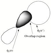
Figure 2.4. Two orbitals' overlap region.
In contrast, the exchange integral
K1,2= ∫ f1(r) f2(r') e2/|r-r'|f2(r) f1(r')dr dr'
can be thought of as a Coulomb repulsion between two electrons whose coordinates r and r' are both distributed throughout the overlap region f1 f2. This overlap region is where both f1 and f2 have appreciable magnitude. This interpretation of exchange integrals as Coulomb interactions between two electrons confined to the overlap region helps us understand why exchange integrals tend to be smaller in magnitude than Coulomb integrals involving the same functions (because the overlap region is a fraction of the total volume of either orbital). It also helps to understand why exchange integrals decay rapidly (and exponentially) with the distance R between the two centers on which the two orbitals are located but Coulomb integrals decay less rapidly (and as 1/R).
As noted above, the Coulomb and exchange integrals in which the two spin-orbital indices are identical cancel (i.e., JI,I = KI,I). This cancellation is important because it assures that the SCF equations do not contain a so-called Coulomb self-interaction of an electron with itself. It may appear obvious that this should be an attribute of any acceptable model for the interactions among electrons, but it turns out that not all commonly used theoretical methods possess it. In particular, most density functional theory (DFT) potentials [[51]] do not guarantee such cancellation in the large-r regions (i.e., where both electrons are far from nuclear centers). As a result, such potentials do not properly yield asymptotic behavior that contains no Coulomb interaction, as should be the case for a singly charged anion. Recall from our earlier discussion about the nature of the long-range attractive and repulsive potentials in neutrals and cations and in anions and multiply charged anions that such potentials differ qualitatively. For these reasons, it is essential to properly describe the large-r behavior of the anion's electron-attracting potential, and thus it is important to use methods that offer this possibility.
III. Koopmans' Theorem Gives the First Approximation to the Electron Affinity
The HF-SCF equations
he fi = ei fi
imply that the SCF orbital enegies ei can be written as:
ei = < fi | he | fi > = < fi | T + V | fi > + Sj(occupied) < fi | Jj - Kj | fi >
= < fi | T + V | fi > + Sj(occupied) [Ji,j - Ki,j ],
where T + V represents the kinetic (T) and nuclear attraction (V) energies, respectively. Thus, ei is the average value of the kinetic energy plus Coulomb attraction to the nuclei for an electron in fi plus the sum over all of the spin-orbitals occupied in Y of Coulomb minus exchange interactions of spin-orbital fi with the other occupied spin-orbitals.
If fi is an occupied spin-orbital, the term [Ji,i - Ki,i ] disappears and the remaining terms in the sum represents the Coulomb minus exchange interaction of fi with all of the N-1 other occupied spin-orbitals. If fi is a virtual spin-orbital, this cancellation does not occur (because j cannot equal i), and one obtains the Coulomb minus exchange interaction of fi with all N of the occupied spin-orbitals in Y. Hence the energies of occupied orbitals pertain to interactions appropriate to a total of N electrons, while the energies of virtual orbitals pertain to a system with N+1 electrons. For this reason, virtual orbitals also tend to be radially more diffuse than occupied orbitals.
Let us consider the following model of the detachment or attachment of an electron in an N-electron system.
- In this model, both the parent molecule and the species generated by adding or removing an electron are treated at the HF level.
- The Hartree-Fock orbitals of the parent molecule are used to describe both species. It is said that such a model neglects 'orbital relaxation' (i.e., the re-optimization of the spin-orbitals to allow them to become appropriate to the daughter anion or cation species).
Within this model, the energy difference between the daughter and the parent can be written as follows (fk represents the particular spin-orbital that is added or removed):
For electron detachment:
EN-1 - EN = - ek ;
For electron attachment:
EN - EN+1 = - ek .
So, within the limitations of the HF, frozen-orbital model, the ionization potentials (IPs) and electron affinities (EAs) are given as the negatives of the occupied and virtual spin-orbital energies, respectively. This statement is referred to as Koopmans' theorem; it is used extensively in quantum chemical calculations as a means of estimating IPs and EAs and often yields results that are qualitatively correct (i.e., ± 0.5 eV) but not usually more accurate than this.
It is useful at this time to reflect a bit more on the physical meaning of the Hartree-Fock orbitals and their energies; let us do so with a concrete example of the N2 molecule. A HF calculation using a reasonable AO basis set on N2 will generate a set of occupied MOs of sg, su, and pu symmetry as well as a set of unoccupied (called virtual) orbitals of sg, su, pg, and pu symmetries. The occupied orbital of pu symmetry corresponds to the bonding p orbital and will have a negative HF orbital energy that, via. Koopmans' theorem, gives an approximation to the energy needed to remove an electron from this orbital:
![]() .
.
However, the lowest-energy unoccupied orbital will not necessarily appear very much like one might expect; that is, it will not necessarily correspond to an anti-bonding pg orbital. Why not? Because the Coulomb and exchange potentials that act on this virtual orbital correpsond to a total of fourteen electrons. This same combination of Coulomb minus exchange potentials acting on, for example, the bonding pu orbital describe only thirteen electrons acting on this orbital. That is, the term
Sj(occupied) [Ji,j - Ki,j ]
in the HF Hamiltonian, when acting on one of the occupied orbitals fo, is of the form
Sj(occupied) [Jo,j - Ko,j ].
In the sum over j, the terms j = o cancel. In contrast, when acting on an unoccupied orbital fu, one obtains
Sj(occupied) [Ju,j - Ku,j ].
Nowhere in the sum over j does the term j = u occur, so one does not obtain the kind of cancellation that occurred in the occupied-orbital case. This means that in and N-electron species, the occupied orbitals feel only the N-1 other electrons' Coulomb and exchange potentials as one expects (i.e., an electron does not experience such an interaction with itself). So, the occupied pu orbital of N2 is an eigenfunction of a Hamiltonian that contains the effects of the remaining thirteen electrons. In contrast, the unoccupied orbitals feel Coulomb and exchange potentials from all N of the occupied orbitals. Hence, the unoccupied pg orbital is an eigenfunction of a Hamiltonian that contains the effects of the fourteen occupied orbitals' electrons. It is for this reason that we often say that virtual HF orbitals are more appropriate for describing the anion (which, of course, is what Koopmans' theorem suggests) while the occupied orbitals more properly relate to the neutral parent.
This example shows that one must be very careful when interpreting virtual orbitals' energies and radial characters. However, it does not answer the question about what one should do if one wants to obtain an orbital of pg symmetry that can be used, for example, to describe a pu1 pg1 state of N2. To approach this problem, one can carry out a separate HF calculation in which the orbitals defined as occupied (i.e., those indexed j in the sum Sj(occupied) [Ji,j - Ki,j]) include one pu and one pgorbital. So, one should use HF orbitals that have been obtained using an occupancy definition that fits the electronic state one wishes to study.
Above, we noted that the virtual orbitals of N2 are more appropriate to the N2- anion than to neutral N2. However, such virtual orbitals cannot be trusted (e.g., their Koompmans' estimate for the EA should not be used) if, as is the case for N2-, the anion is electronically metastable with respect to electron autodetachment. In such cases, the specialized techniques detailed in Section IV of Chapter 5 need to be employed to gain even a qualitatively correct description of the metastable anion's orbitals.
IV. Electron Correlation Involving the Excess Electron Usually Must be Treated
To achieve reasonable chemical accuracy (e.g., ± 5 kcal/mole) in electronic structure calculations, one cannot describe the wave function Y in terms of a single determinant as is done in the Hartree-Fock approach. Above and beyond cases such as the 1S state of the carbon atom discussed earlier in which three determinants are needed just to form a function of proper spin and spatial symmetry, there are other situations in which more than one determinant should be used. The reason a single-determinant wave function is inadequate for all species when one desires high accuracy is because the spatial probability density functions are not correlated when such a function is used. In other words, the probability P(r,r') of finding one electron at point r and a second electron at r' for a single-determinant wave function turns out as we show later to be the product p(r) of finding one electron at r times the probability p(r') of finding an electron at r' P(r,r') = p(r) p(r'). This means the probability of finding one electron at position r is independent of where the other electrons are, which is absurd because the electrons' mutual Coulomb repulsion causes them to avoid one another.
This mutual avoidance is what we call electron correlation because the electrons' motions as reflected in their spatial probability densities are correlated (i.e., inter-related). It turns out that the differences between predictions of non-correlated (e.g., Hartree-Fock) and correlated theories of EAs are quite substantial and often amount to ca. 0.5 eV, so it is essential that one use correlated methods to achieve reliable EAs.
Let us consider a simple example to illustrate this problem with single determinant functions. The |1sa(r) 1sb(r')| determinant appropriate, for example to a He atom, when written as
|1sa(r) 1sb(r')| = 2-1/2{1sa(r) 1sb(r') - 1sa(r') 1sb(r)}
can be multiplied by itself to produce the 2-electron probability density:
P(r, r') = 1/2{[1sa(r) 1sb(r')]2 + [1sa(r') 1sb(r)]2
-1sa(r) 1sb(r') 1sa(r') 1sb(r) - 1sa(r') 1sb(r) 1sa(r) 1sb(r')}.
If we now integrate over the spins of the two electrons and make use of the orthonormality of the a and b spin functions
<a|a> = <b|b> = 1, and <a}b> = <b}a> = 0,
we obtain the following spatial (i.e., with spin absent) probability density:
P(r,r') = |1s(r)|2 |1s(r')|2.
This probability, being a product of the probability density for finding one electron at r times the density of finding another electron at r', clearly has no correlation in it. That is, the probability of finding one electron at r does not depend on where (r') the other electron is. This product form for P(r,r') is a direct result of the single-determinant form for Y, so this form must be wrong if electron correlation is to be accounted for. In fact, the Coulomb repulsions between pairs of electrons causes the true pair distribution function P(r,r') to vanish as r approaches r'. In fact, P(r,r') has a cusp whenever |r – r'| 0; unlike the cusp in the electronic wave functions at geometries where r approaches a nuclear center (n.b., this probability density is non-vanishing at the nuclear center where it has a non-zero slope), the electron-pair probability vanishes at |r – r'| = 0 and has a non-zero slope.
Now, we need to ask how Y should be written if such correlation effects are to be taken into account. One approach is to introduce into the form of the ansatz wave function terms that depend explicitly on the inter-electron coordinates ri,j and to cast these terms in a way that causes the wave function to decay whenever any ri,j becomes small. Such so-called explicitly correlated approaches are indeed possible to use, but, because of the added complexity that such functional forms introduce into their practical implementations, their use currently is limited to rather small molecules and ions. Therefore, it is more common (and practical) to use other means to allow the electrons to avoid one another and it is such approaches that we shall focus on here.
It turns out that one can account for electron avoidance (for each pair of electrons) by taking Y to be a combination of two or more determinants that differ by the promotion of two electrons from one orbital to another orbital (i.e., from an occupied orbital to a so-called virtual orbital-one that is not occupied in the more approximate wave function). In such a wave function, we say that doubly excited determinants have been included, and the approach of combining two or more determinants to form a wave function is called configuration interaction (CI).
For example, in describing the p2 bonding electron pair of an olefin or the ns2 electron pair in alkaline earth atoms, we find it important to mix in doubly excited determinants of the form (p*)2 or np2, respectively. It turns out that the avoidance of electrons that occupy the same orbital are the most important to include (i.e, have the largest energy contribution), but correlations between electrons occupying different orbitals (e.g., 1s 2s electron correlation in Be) are also important if one wishes to achieve high accuracy.
Briefly, the physical importance of such doubly-excited determinants can be made clear by using the following identity involving the combination of any pair of determinants denoted | ..fa fb..| and | ..f'a f'b..| that differ by only two spin-orbitals (fa and fb vs. f'a and f'b) :
Y = C1 | ..fa fb..| - C2 | ..f'a f'b..|
= C1/2 { | ..( f - xf')a ( f + xf')b..| - | ..( f - xf')b ( f + xf')a..| },
where
x = (C2/C1)1/2 .
This identity allows one to interpret the combination (C1 | ..fa fb..| - C2 | ..f'a f'b..|) of two determinants that differ from one another by a double promotion from one orbital (f) to another (f') as equivalent to a singlet coupling (i.e., having 2-1/2 (ab-ba) spin function) of two different orbitals (f - xf') and (f + xf'). Let us now see how this identity helps us understand how such CI wave functions can incorporate correlations among the electrons' motions.
In the olefin example mentioned above, the two non-orthogonal polarized orbital pairs
(f - xf') and (f + xf') involve mixing the f = p and f' = p* orbitals to produce two
left-right polarized orbitals as depicted in Fig. 2.5.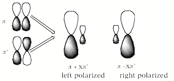
Figure 2.5. Polarized p orbital pairs.
In this case, one says that the p2 electron pair undergoes left-right correlation when the (p*)2 determinant is mixed into the CI wave function. One electron is in p+xp* on the left while the other is in p-xp* on the right.
In the alkaline earth atom case, the polarized orbital pairs are formed by mixing the ns and np orbitals (actually, one must mix in equal amounts of px, py , and pz orbitals to preserve overall 1S symmetry in this case), which gives rise to angular correlation of the electron pair. Such a pair of polarized orbitals is shown in Fig. 2.6.
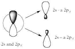
Figure 2.6. Polarized s and p orbital pairs.
More specifically, the following four determinants are included to form polarized orbital pairs and to preserve the 1S spin and orbital angular momentum character in Y:
Y = C1 |1s22s2 | - C2 [|1s22px2 | +|1s22py2 | +|1s22pz2 |].
The fact that the latter three terms possess the same amplitude C2 is a result of the requirement that a state of 1S symmetry is involved. It can be shown that this four-determinant function is equivalent to:
Y = 1/6 C1 |1sa1sb{[(2s-a2px)a (2s+a2px)b - (2s-a2px)b(2s+a2px)a]
+[(2s-a2py)a(2s+a2py)b - (2s-a2py)b(2s+a2py)a]
+[(2s-a2pz)a(2s+a2pz)b - (2s-a2pz)b(2s+a2pz)a] |,
where a = (3C2/C1)1/2. Here two electrons occupy the 1s orbital (with opposite, a and b spins) and are thus treated in a non-correlated manner while the other pair resides in 2s-2p polarized orbitals in a manner that instantaneously correlates their motions. This illustrates that wave functions can be created which correlate selected subsets of the occupied spin-orbitals while treating others at the non-correlated level.
The polarized orbital pairs (2s ± a 2px,y, or z) are formed by combining the 2s orbital with the 2px,y, or z orbital in a ratio determined by C2/C1. As we will see later when we deal with how to evaluate Hamiltonian matrix elements between pairs of determinental wave functions, this ratio C2/C1 can be shown to be proportional to the magnitude of the coupling matrix element
<1s22s2 |H|1s22p2 >
between the two determinants involved and inversely proportional to the energy difference
[<1s22s2H|1s22s2> - <1s22p2|H|1s22p2>]
between these configurations. In general, configurations that have similar Hamiltonian expectation values and that are coupled strongly give rise to strongly mixed (i.e., with large |C2/C1| ratios) polarized orbital pairs.
In each of the three equivalent terms in the above alkaline earth wave function, one of the valence electrons moves in a 2s+a2p orbital polarized in one direction (x, y, or z) while the other valence electron moves in the 2s-a2p orbital polarized in the opposite x, y, or z direction. For example, the first term
[(2s-a2px)a(2s+a2px)b] - (2s-a2px)b(2s+a2px)a]
describes one electron occupying a 2s-a2px polarized orbital while the other electron occupies the 2s+a2px orbital. The electrons thus reduce their Coulomb repulsion by occupying different regions of space; in the SCF picture 1s22s2, both valence electrons reside in the same 2s region of space. In this particular example, the electrons undergo angular correlation to 'avoid' one another. To achieve an even higher-level description of angular correlation, one can also employ functions with angular momentum higher than the p-functions described above. That is, L=2, 3, ... basis functions can be used to gain an even more accurate description of angular correlation.
The use of doubly excited determinants is thus seen to be a mechanism by which Y can place electron pairs, which in the single-configuration picture occupy the same orbital, into different regions of space (i.e., each one into a different member of the polarized orbital pair) thereby lowering their mutual Coulomb repulsion. Such electron correlation effects are referred to as dynamical electron correlation; they are extremely important to include if one expects to achieve chemically meaningful accuracy (i.e., ± 5 kcal/mole). As mentioned earlier, because molecular EAs can be of this order of magnitude, their accurate calculation usually requires one to include such dynamical electron correlation effects.
In practical quantum chemistry calculations on anions, one must compute the C2/C1 ratios (more appropriately, all of the CI coefficients in the CI expansion of Y
Y = SJ CJ FJ,
where the FJ are spin and spatial symmetry adapted configuration state functions (i.e., combinations of Slater determinants that produce the proper spin and space symmetry).There are a variety of approaches that can be used to compute the CI coefficients as well as the energy E. The most commonly employed methods are the configuration interaction (CI), Møller-Plessset (MP) perturbation, and coupled-cluster (CC) methods. Each has strengths and weaknesses that we briefly review in the following subsection.
V. Various Methods Can be Used to Treat Correlation
There are numerous procedures currently in use for determining the 'best' wave function of the form:
Y = SI CI FI,
where FI is a spin-and space- symmetry-adapted configuration state function (CSF) consisting of linear combinations of determinants each of which we denote | fI1 fI2 fI3 ... fIN | in terms of their N occupied spin-orbitals. In all such wave functions, there are two kinds of parameters that need to be determined- the CI coefficients and the LCAO-MO coefficients describing the fIk . Because treatment of electron correlation is an integral part of nearly all studies of molecular anions, it is important to survey the variety of approaches that are used for this purpose.
The most commonly employed methods used to determine these parameters include:
A. The multiconfigurational self-consistent field (MCSCF) method
In this approach, the expectation value < Y | H | Y > / < Y | Y > is treated variationally and made stationary with respect to variations in both the CI and Ci,n coefficients. The energy functional is a quadratic function of the CI coefficients, and so one can express the stationary conditions for these variables in terms of a matrix eigenvalue problem:
SJ HI,J CJ = E CI .
However, E is a quartic function of the Ci,n 's because, as we will show later, each HI,J matrix element can be expressed in terms of two-electron integrals <fifj | g |fkfl> each of which depend quartically on the Cn,i coefficients because each fj is a linear combination of bais orbitals cn multiplied by Ci,n.
In the MCSCF method the number of CSFs is usually kept to a small to moderate number (e.g., a few to several thousand) chosen to describe essential correlations (i.e., configuration crossings, near degeneracies, proper dissociation, all of which are often termed non-dynamical correlations) and important dynamical correlations (those electron-pair correlations of angular, radial, left-right, etc. nature that are important to the anion-neutral energy difference). For the alkaline earth example used earlier, the four determinants in the two-CSF wave function Y = C1 |1s22s2 | - C2 [|1s22px2 | +|1s22py2 | +|1s22pz2 |] could be used to carry out an MCSCF calculation in which case one would speak of including angular dynamical correlations of the electrons occupying the two 2s spin-orbitals.
B. The configuration interaction (CI) method
In this approach, the LCAO-MO coefficients of all the spin-orbitals are determined first via a single-configuration SCF calculation or an MCSCF calculation using a small number of CSFs. The CI coefficients are subsequently determined by making the energy expectation value < Y | H | Y > / < Y | Y > stationary. The CI wave function is most commonly constructed from CSFs FJ that include:
- All of the CSFs in the SCF or MCSCF wave function that was used to generate the molecular spin-orbitals fi. These are referred to as the 'reference' CSFs. For the alkaline earth example, the four determinants in Y = C1 |1s22s2 | - C2 [|1s22px2 | +|1s22py2 | +|1s22pz2 |] might constitute such a list of two reference CSFs.
- CSFs generated by carrying out single, double, triple, etc. level 'excitations' (i.e., orbital replacements) relative to reference CSFs. For the alkaline earth example, determinants of the form 1s2ns2|, ms22s2|, 1s2np2 |, and 1s223d2 | (with n, m ³ 3) might be included. CI wave functions limited to include contributions through various levels of excitation are denoted S (singly), D (doubly), SD (singly and doubly), SDT (singly, doubly, and triply) excited.
As we already introduced, the orbitals from which electrons are removed can be restricted to focus attention on correlations among certain orbitals. For example, if excitations out of core electrons are excluded, one computes a total energy that contains no core correlation energy. The number of CSFs included in the CI calculation is often far in excess of the number considered in an equivalent-quality MCSCF wave function (because in the latter, one also optimizes the LCAO-MO coefficients). CI wave functions including 5,000 to 50,000 CSFs are routine, and functions with one to several billion CSFs are within the realm of practicality.
The need for such large CSF expansions in a CI wave function might be surprising but is relatively easy to understand. Consider (i) that each electron pair requires at least two CSFs to form polarized orbital pairs that can correlate their motions, (ii) there are of the order of N(N-1)/2 electron pairs for N electrons, hence (iii) the number of terms in the CI wave function scales as 2N(N-1)/2. For a molecule containing ten electrons, there thus could be 245 = 3.5 x10¹³ terms in the CI expansion. This may be an over estimate of the number of CSFs needed, but it demonstrates how rapidly the number of CSFs can grow with the number of electron pairs that one wishes to correlate.
i. The Slater-Condon Rules
In all of the methods used to treat electron correlation, the HI,J matrices are, in practice, evaluated in terms of one- and two- electron integrals over the molecular orbitals using the so-called Slater-Condon rules or their equivalent. These rules express all non-vanishing matrix elements involving either one- or two- electron operators between any pair of determinental wave functions in which the constituent spin-orbitals are orthonormal. One-electron operators (e.g., the kinetic energy and the electron-nuclei Coulomb attraction potentials) are one-electron additive and appear in any quantum mechanical operator, including the Hamiltonian, as
F = Si f(i).
Two-electron operators (e.g., the electron-electron Coulomb repulsions) are pair wise additive and always appear as
G = Sij g(i,j)).
The Slater-Condon rules give the matrix elements between any two determinants
| > = |f1f2f3... fN|
and
| ' > = |f'1f'2f'3...f'N|
for any quantum mechanical operator that is a sum of one- and two- electron operators (F + G). It expresses these matrix elements in terms of one-and two-electron integrals involving the spin-orbitals that appear in | > and | ' > and the operators f and g.
As a first step in applying these rules, one must examine | > and | ' > and determine by how many (if any) spin-orbitals | > and | ' > differ. In so doing, one may have to reorder the spin-orbitals in one of the determinants to achieve maximal coincidence with those in the other determinant; it is essential to keep track of the number of permutations (Np) that one makes in achieving maximal coincidence. The results of the Slater-Condon rules given below are then multiplied by (-1)Np to obtain the matrix elements between the original | > and | ' >. The final result does not depend on whether one chooses to permute | > or | ' >.
The Hamiltonian is, of course, a specific example of such an operator; the electric dipole operator Si eri and the electronic kinetic energy - n2/2meSi∇i2 are examples of one-electron operators (for which one takes g = 0); the electron-electron coulomb interaction Si>j e2/rij is a two-electron operator (for which one takes f = 0). Once maximal coincidence has been achieved, the Slater-Condon (SC) rules provide the following prescriptions for evaluating the matrix elements of any operator F + G containing a one-electron part F = Si f(i) and a two-electron part G = Sij g(i,j).:
(i) If | > and | ' > are identical, then
< | F + G | > = Si < fi | f | fi > +Si>j [< fifj | g | fifj > - < fifj | g | fjfj >],
where the sums over i and j run over all spin-orbitals in | >;
(ii) If | > and | ' > differ by a single spin-orbital mismatch ( fp ≠ f'p ),
< | F + G | ' > = < fp | f | f'p > +Sj [< fpfj | g | f'pfj > - < fpfj | g | fjf'p >],
where the sum over j runs over all spin-orbitals in | > except fp ;
(iii) If | > and | ' > differ by two spin-orbitals ( fp ≠ f'p and fq ≠ f'q):
< | F + G | ' > = < fp fq | g | f'p f'q > - < fp fq | g | f'q f'p >
(note that the F contribution vanishes in this case);
(iv) If | > and | ' > differ by three or more spin orbitals, then
< | F + G | ' > = 0;
(v) For the identity operator I, the matrix elements < | I | ' > = 0 if | > and | ' > differ by one or more spin-orbitals (i.e., the Slater determinants are orthonormal if their spin-orbitals are).
Recall that each of these results is subject to multiplication by a factor of (-1)Np to account for possible ordering differences in the spin-orbitals in | > and | ' >. In these expressions,
< fi | f | fj >
is used to denote the one-electron integral
∫ f*i(r) f(r) fj(r) dr
and
< fifj | g | fkfl >
(or in short hand notation < i j| k l >) represents the two-electron integral
∫ f*i(r) f*j(r') g(r,r') fk(r)fl(r') dr dr'.
The short-hand notation < i j | k l> is often used to express the two-electron integrals for the g(r,r') operator in the so-called Dirac notation, in which the i and k indices label the spin-orbitals that refer to the coordinates r and the j and l indices label the spin-orbitals referring to coordinates r'. The r and r' denote r,q,f,s and r',q',f',s' (with s and s' being the a or b spin functions). If the operators f and g do not contain any electron spin operators, then the spin integrations implicit in these integrals (all of the fi are spin-orbitals, so each f is accompanied by an a or b spin function and each f* involves the adjoint of one of the a or b spin functions) can be carried out as <a|a> =1, <a|b> =0, <b|a> =0, <b|b> =1, thereby yielding integrals over spatial orbitals.
ii. The AO-to-MO Integral Transformation
Prior to forming the HI,J matrix elements using such rules, the one- and two- electron integrals, which can be computed only for the atomic (e.g., STO or GTO) basis (e.g. the two-electron Coulomb integrals in the AO basis < cicj | g | ckcl > can be computed), must be transformed to the molecular orbital basis to obtain the integrals
< fifj | g | fkfl > in terms of MOs. This integral transformation step, which involves using the LCAO-MO expansion fj = SmCj,m cm, requires computer resources proportional to the fifth power of the number of basis functions, and thus is one of the more troublesome steps in most configuration interaction and other correlated-level calculations. This transformation is performed in four steps. In the first, the AO integrals are transformed to an intermediate set of integrals whose indices refer to three AOs and one MO:
< cicj | g | ckfm> = Sl Cm,l < cicj | g | ckcl >.
This so-called one-index transformation requires computational effort proportional to N5 (e.g., imagine four do-loops over i, j, k, and m and then a sum loop over l). After the
< cicj | g | ckfm> array is formed, one carries out a second one-index transformation to form the < cicj | g | fnfm> list. The series of four such one-index transformations ultimately leads to the desired < fifj | g | fkfl > integral list with a total effort proportional to N5.
C. The Møller-Plesset perturbation (MPPT) method
This method uses the single-configuration SCF process to determine a set of spin-orbitals {fi}. Then, using an unperturbed Hamiltonian equal to the sum of the N electrons' Fock operators H0 = Si=1,N F(i), perturbation theory is used to determine the CI amplitudes for the CSFs. The amplitude for the reference CSF F is taken as unity and the other CSFs' amplitudes are determined by Rayleigh-Schrödinger perturbation using H-H0 as the perturbation.
Actually, in the most common version of MPPT, a single determinant containing N spin-orbitals is used as the reference function.
In the MPPT method, once the reference CSF is chosen and the SCF orbitals belonging to this CSF are determined, the wave function Y and energy E are determined in an order-by-order manner. The perturbation equations determine which CSFs to include through any particular order. This is one of the primary strengths of this technique; it does not require one to make choices of which configurations to include, in contrast to the MCSCF and CI treatments where one needs to choose the CSFs.
For example, the first-order wave function correction Y1 is:
Y1 = - Si<j,m<n [< i,j |g| m,n > -< i,j |g| n,m >][ em-ei +en-ej ]-1 | Fi,jm,n >,
where the SCF orbital energies are denoted ek and Fi,jm,n represents a CSF that is doubly excited (fi and fj are replaced by fm and fn) relative to the zeroth-order wave function F. Note that it is doubly excited determinants that are the most important contributors beyond the zeroth-order single determinant; this observation supports the notions put forth earlier that forming polarized orbital pairs is an important and efficient way to allow for electron correlation effects. The reason that singly-excited determinants are not important (at least through first order) can be understood by noting that the sum of a single zeroth-order determinant |f1f2f3..fa.fN| and a singly-excited determinant |f1f2f3..fp.fN| in which spin-orbital fa is replaced by fp can be rewritten as another single determinant:
|f1f2f3..fa.fN| + x |f1f2f3..fp.fN| = |f1f2f3..(fa +xfp).fN| .
So, any inclusion of singly-excited determinants can be viewed as equivalent to variations in the spin-orbitals themselves. However, by assumption, the Hartree-Fock SCF process has been used to optimize (i.e., make the energy minimum) the spin-orbitals, so if the fJ used to form the zeroth-order single determinant are HF spin-orbitals, then there is no need to vary them further. In other words, the optimum value for the parameter x shown in the equation above is x = 0. This observation, that singly-excited determinants have zero amplitudes in the MPPT wave function (to first order) is known as the Brillouin theorem.
Once the wave function is known to first order as above, the energy E can be computed through second order where it is given as:
E = <F|H0 + V|F + Y1> = ESCF - Si<j,m<n | < i,j | g | m,n > -
< i,j | g | n,m > |2/[ em-ei +en -ej ].
Both Y and E are expressed in terms of two-electron integrals < i,j |g| m,n > coupling the virtual spin-orbitals fm and fn to the spin-orbitals from which electrons were excited fi and fj as well as the orbital energy differences [em-ei +en -ej ] accompanying such excitations. Clearly, as we stated earlier in discussing the angular correlations in the alkaline earth atoms, major contributions to the correlation energy are made by double excitations into virtual orbitals fm fn with large < i,j | g | m,n > integrals and small orbital energy gaps [em-ei +en -ej]. In higher order corrections, contributions from CSFs that are singly, triply, etc. excited relative to F appear, and additional contributions from the doubly excited CSFs also enter.
D. The Coupled-Cluster (CC) method
In this method, one expresses the wave function in a somewhat different manner:
Y = exp(T) F,
where F is a single CSF (usually the single determinant) used in the SCF process to generate a set of spin-orbitals. The operator T is expressed in terms of operators that achieve spin-orbital excitations as follows:
T = Si,m tim m+ i + Si,j,m,n ti,jm,n m+ n+ j i + ...,
where the combination of operators m+ i denotes creation of an electron in virtual spin-orbital fm and removal of an electron from occupied spin-orbital fi to generate a single excitation. The operation m+ n+ j i therefore represents a double excitation from fi fj to fm fn. When carrying out CC calculations in which only m+ i operators are employed, one speaks of performing a CCS calculations with the S denoting that only single excitation operators are used. Likewise, CCSD calculations would include both m+ i and m+ n+ j i operators, while CCSDT calculations also include the triple-excitation operators.
The amplitudes tim , ti,jm,n, etc., which play the role of the CI coefficients in CC theory, are determined through the set of equations generated by projecting the Schrödinger equation in the form (this is obtained by multiplying H exp(T) F = E exp(T) F on the left by exp(-T))
exp(-T) H exp(T) F = E F
against CSFs which are single, double, etc. excitations relative to F:
< Fim | H + [H,T] + 1/2 [[H,T],T] + 1/6 [[[H,T],T],T] + 1/24 [[[[H,T],T],T],T] | F > = 0;
< Fi,jm,n |H + [H,T] + 1/2 [[H,T],T] + 1/6 [[[H,T],T],T] + 1/24 [[[[H,T],T],T],T] |F> =0;
< Fi,j,km,n,p|H + [H,T] + 1/2[[H,T],T] + 1/6 [[[H,T],T],T] + 1/24 [[[[H,T],T],T],T] |F> = 0,
and so on for higher order excited CSFs. It can be shown that the expansion of the exponential operators that generates the various commutators shown above truncates exactly at the fourth power in T. As a result, the exact CC equations are quartic equations for the tim , ti,jm,n , etc. amplitudes. The matrix elements appearing in the CC equations can be expressed (e.g., using the Slater-Condon rules) in terms of one- and two- electron integrals over the spin-orbitals including those occupied in F and the virtual orbitals not in F.
These quartic equations are solved in an iterative manner and, as such, are susceptible to convergence difficulties that can plague any such scheme. In such iterative processes, it is important to start with an approximation reasonably close to the final result. In CC theory, this is often achieved by initially neglecting all of the terms that are non-linear in the t amplitudes (because the t's are assumed to be less than unity in magnitude) and ignoring factors that couple different doubly excited CSFs (i.e., the sum over i',j',m',n'). This gives t amplitudes that are equal to the amplitudes of the first-order MPPT wave function:
ti,jm,n = - < i,j | g | m,n >'/ [ em-ei +en -ej ] .
Although the CC method involves equations that must be solved iteratively, it is one of the most accurate and reliable tools available to the theoretical study of molecular anions.
One of the strengths of CC theory is its ability to represent reasonably accurately the contributions of excitations higher than double excitations to the correlated movements of the electrons in a multi-electron molecule. For example, even when including in the cluster operator T only double excitations { m+ n+ j i}, the CC wave function exp(T) F contains contributions from double, quadruple, sextuple, etc. excited determinants:
exp(T) F = {1 + Sm,n,Iij tm,n,i,j m+ n+ j i + 1/2 (Sm,n,Iij tm,n,i,j m+ >n+ j i)( Sm,n,Iij ti,jm,nm+ n+ j i)
+ 1/6 (Sm,n,Iij ti,jm,nm+ n+ j i) (Sm,n,Iij ti,jm,nm+ n+ j i) (Sm,n,Iij ti,jm,nm+ n+ j i) + ...}F.
In such a function, the amplitudes of, for example, the quadruply-excited determinants m+ n+ j i p+ q+ lk F are given in terms of products of the amplitudes of the constituent doubly-excited determinants ti,jm,ntk,lp,q rather than as independent parameters tp,q,k,lm,n,i,j. Is this a good or a bad thing? It turns out that even when, in a CI calculation, the doubly-, quadruply-, sextuply- etc. level excitations are included with independent amplitudes in the wave function, the resultant amplitudes of the quadruply- and sextuply- excited determinants are indeed approximately equal to products of the constituent doubly-excited determinants' amplitudes.
This observation, that excitations of order 2P have amplitudes nearly equal to the products of the amplitudes of the P double excitations comprising the 2P-order excitation, suggests that independent (so-called unlinked) pair wise correlations of electrons dominate over three- or higher- electron correlations. For example, when four electrons undergo correlated motions, the largest contributions arise from one pair of electrons interacting and avoiding one another in one region of space while a second pair (not spatially close to the first pair) is avoiding one another somewhere else. Contributions in which one electron pair is interacting while another pair is nearby (i.e., so-called linked contributions) are found to be less important to consider. This is very reminiscent of what is found in low-order virial expansions of dense-gas partition functions. One finds that four-body correlation functions P(r1,r2,r3,r4) are nearly equal to products of two-body correlation functions P(r1,r2) P(r3,r4) because, at modest densities, the chances that three or four molecules are simultaneously near one another is much smaller than the chances that two molecules are close to one another while another two are near one another but not close to the first pair.
The vast majority of studies of electron affinities and of negative molecular ions carried out by Professor Ernest Davidson and Professor Fritz Schaefer have made use of the MCSCF, CI, or CC approaches. These two scientists have made many important contributions to the development and implementation of all three of these methods.
E. Density Functional Theory (DFT)
The density functional approaches provide alternatives to the conventional tools of quantum chemistry. The CI, MCSCF, MPPT, and CC methods move beyond the single-configuration picture by adding to the wave function more configurations whose amplitudes they each determine in their own way as outlined above. This can lead to a very large number of CSFs in the correlated wave function, and, as a result, a need for extraordinary computer resources.
However, there is a special difficulty with the current state of the art in DFT as far as anions are concerned. At present, almost all of the functionals that are used in DFT to express the interaction potential that an electron experiences have an incorrect form when the electron's radial coordinate r is large. Specifically, in such asymptotic regions, the functionals contain terms that are attractive and vary with r as –a/r; that is, they show a Coulomb-like attraction. As we discussed in Section I, an electron in a mono-anion experiences at large-r no such Coulomb potential; nor does an electron in a multiply-charged anion. For this reason, it is dangerous to use DFT methods with such functionals when studying anions, especially anions with very small EAs. It is for such species that significant electron density exists at large-r where the functionals are incorrect. We should note, however, that calculations of EAs with DFT methods can be reasonably accurate, especially when the anion's charge density is rather compact (i.e., when the EA is large). For example, in the latest tabulation of atomic and molecular EAs [4] essentially all of the theoretical EAs quoted (n.b., ref. 4 also contains a large number of experimentally determined EAs) were obtained using DFT methods. One can gain an appreciation for the reliability of DFT in studying anions by perusing the data contained in that reference.
Let us now discuss what DFT is and how it has been developed. The density functional approaches are different [51] from the wave function theories we have reviewed so far. Here one solves a set of orbital-level equations
[ - >h2/2m 2 - SA ZAe2/|r-RA| + ![]() + U(r)] fi = ei fi
+ U(r)] fi = ei fi
in which the orbitals {fi} 'feel' potentials due to the nuclear centers (having charges ZA), Coulomb interaction with the total electron density r(r'), and a so-called exchange-correlation potential denoted U(r'). The particular electronic state for which the calculation is being performed is specified by forming a corresponding density r(r'). Before going further in describing how DFT calculations are carried out, let us examine the origin of the fundamental ideas underlying this theory.
The so-called Hohenberg-Kohn theorem states that the ground-state electron density r(r) describing any N-electron system uniquely determines the potential V(r) in the Hamiltonian
H = Sj {-h2/2m ∇j2 + V(rj) + e2/2 Sk≠j 1/rj,k },
and, because H determines the energies and wave functions of the system, the ground-state density r(r) thus determines all the properties of the system. The proof of this theorem proceeds as follows:
Suppose one knows an electron density r(r) at all points in space r. Then,
- r(r) can be used to determine the number of electrons N in the system through
∫ r(r) d3r = N. - But how do r(r) and N determine the Hamiltonian H? If one knows N, one can certainly write down the kinetic and electron-electron repulsion parts of H as Sj {-h2/2me ∇j2 + e2/2 Sk≠j 1/rj,k }, but how does one figure out the V(r) = Sj V(rj) part of H? After all, it is this component of H that depends on where the nuclei are located and on any external fields that are present.
- Assume that there are two distinct potentials (aside from an additive constant that simply shifts the zero of total energy) V(r) and V'(r) which form two Hamiltonians H and H', respectively having the same number of electrons but differing only in V and V'. Further, assume one uses H and H' to solve the Schrödinger equation for their respective ground-state energies and wave functions E0, Y (r) and E0', Y' (r). Finally, assume that Y and Y' have the same one-electron density: ∫ |Y|2 dr2 dr3 ... drN = r(r) = ∫ |Y'|2 dr2 dr3 ... drN .
- If we think of Y' as trial variational wave function for the Hamiltonian H, we know
that
E0 < <Y'|H|Y'> = <Y'|H'|Y'> + ∫r(r) [V(r) - V'(r)] d3r = E0' + ∫r(r) [V(r) - V'(r)] d3r. - Similarly, taking Y as a trial function for the H' Hamiltonian, one finds that
E0' < E0 + ∫r(r) [V'(r) - V(r)] d3r. - Adding the equations in d and e gives
E0 + E0' < E0 + E0',
which is a clear contradiction.
Hence, our assumption that there are two distinct potentials V and V' that give the same ground-state density r(r) must be incorrect. So, for a given ground-state density r (r), there is only one unique potential V(r). This means that r(r) determines N and a unique V, and thus determines H, and therefore all Ys and all Es. Furthermore, because Y determines all properties, then r(r), in principle, determines all such properties.
This means that even the kinetic energy and the electron-electron interaction energy are determined by r(r). It is easy to see that ∫r (r) V(r) d3r = V[r] gives the average value of the electron-nuclear (plus any additional one-electron additive potential) interaction in terms of the ground-state density r(r), but how are the kinetic energy T[r] and the electron-electron interaction Vee[r] energy expressed in terms of r?
The main difficulty with DFT is that the Hohenberg-Kohn theorem shows that the values of T, Vee, V, etc. are all unique functionals of the ground-state r (i.e., that they can, in principle, be determined once r is given), but it does not tell us what these functional relations are.
To see how it might make sense that a property such as the kinetic energy, whose operator -h2 /2me ∇2 involves derivatives, can be related to the electron density, consider a simple system of N non-interacting electrons moving in a three-dimensional cubic box potential. The energy states of such electrons are known to be
E = (h2/2mL2) (nx2 + ny2 +nz2),
where L is the length of the box along the three axes, and nx , ny , and nz are the quantum numbers describing the state. We can view nx2 + ny2 +nz2 = R2 as defining the squared radius of a sphere in three dimensions, and we realize that the density of quantum states in this space is one state per unit volume in the nx , ny , nz space. Because nx , ny , and nz must be positive integers, the volume covering all states with energy less than or equal to a specified energy E = (h2/2meL2) R2 is 1/8 the volume of the sphere of radius R:
F(E) = 1/8 (4p/3) R3 = (p/6) (8mL2E/h2)3/2 .
Since there is one state per unit of such volume, F(E) is also the number of states with energy less than or equal to E, and is called the integrated density of states. The number of states g(E) dE with energy between E and E+dE, the density of states, is the derivative of F:
g(E) = dF/dE = (p/4) (8mL2/h2)3/2 E1/2 .
If we calculate the total energy for N electrons, with all the states having energies up to the so-called Fermi energy (i.e., the energy of the highest occupied molecular orbital HOMO) being doubly occupied, we obtain the ground-state energy:
E0 = 2 ![]() g(E) E dE = (8p/5) (2m/h2)3/2 L3 EF5/2.
g(E) E dE = (8p/5) (2m/h2)3/2 L3 EF5/2.
The total number of electrons N can be expressed as
N = 2 ![]() g(E) dE = (8p/3) (2m/h2)3/2 L3 EF3/2,
g(E) dE = (8p/3) (2m/h2)3/2 L3 EF3/2,
which can be solved for EF in terms of N to then express E0 in terms of N instead of EF:
E0 = (3h2/10m) (3/8p)2/3 L3 (N/L3)5/3 .
This gives the total energy, which is also the kinetic energy in this case because the potential energy is zero within the box, in terms of the electron density r (x,y,z) = (N/L3). It therefore may be plausible to express kinetic energies in terms of electron densities r(r), but it is by no means clear how to do so for real atoms and molecules with electron-nuclear and electron-electron interactions operative.
In one of the earliest DFT models, the Thomas-Fermi theory, the kinetic energy of an atom or molecule is approximated using the above kind of treatment on a local level. That is, for each volume element in r-space, one assumes the expression given above to be valid, and then one integrates over all r to compute the total kinetic energy:
TTF[r] = ∫ (3h2/10m) (3/8p)2/3[r(r)]5/3 d3r = CF ∫ [r(r)]5/3 d3r ,
where the last equality simply defines the CF constant (which is 2.8712 in atomic units where the atomic unit of energy, the Hartree, is 27.21 eV and the unit of length, the Bohr is 0.529 Å). Ignoring the correlation and exchange contributions to the total energy, this T is combined with the electron-nuclear V and Coulomb electron-electron potential energies to give the Thomas-Fermi total energy:
E0,TF [r] = CF ∫[r(r)]5/3 d3r + ∫ V(r) r(r) d3r + e2/2 r(r) r(r')/|r-r'| d3r d3r',
This expression is an example of how E0 is given as a local density functional approximation (LDA). The term local means that the energy is given as a functional (i.e., a function of r) that depends only on r(r) at points in space but not on r(r) at more than one point in space or, equivalently, on derivatives of r(r).
Unfortunately, the Thomas-Fermi energy functional does not produce results that are of sufficiently high accuracy to be of great use in chemistry. What is missing in this theory are the exchange energy and the correlation energy; moreover, the kinetic energy is treated only in the approximate manner described.
In the book by Parr and Yang [51], it is shown how Dirac was able to address the exchange energy for the 'uniform electron gas' (N Coulomb interacting electrons moving in a uniform positive background charge whose magnitude balances the charge of the N electrons). If the exact expression for the exchange energy of the uniform electron gas is applied on a local level, one obtains the commonly used Dirac local density approximation to the exchange energy:
Eex,Dirac[r] = - Cx ∫[r(r)]4/3 d3r,
with Cx = (3/4) (3/p)1/3 = 0.7386 in atomic units. Adding this exchange energy to the Thomas-Fermi total energy E0,TF [r] gives the so-called Thomas-Fermi-Dirac (TFD) energy functional.
Because electron densities vary rather strongly spatially near the nuclei, corrections to the above approximations to T[r] and Eex.Dirac are needed. One of the more commonly used so-called gradient-corrected approximations is that invented by Becke [[52]], and referred to as the Becke88 exchange functional:
Eex(Becke88) = Eex,Dirac[r] -g ∫x2 r4/3 (1+6 g x sinh-1(x))-1 dr,
where x =r-4/3 |∇r|, and g is a parameter chosen so that the above exchange energy can best reproduce the known exchange energies of specific electronic states of the inert gas atoms (Becke finds g to equal 0.0042). A common gradient correction to the earlier T[r] is called the Weizsacker correction and is given by
dTWeizsacker = (1/72)(ħ/m) ∫|∇r(r)|2/r(r) dr.
Although the above discussion suggests how one might compute the ground-state energy once the ground-state density r(r) is given, one still needs to know how to obtain r. Kohn and Sham [[53]] (KS) introduced a set of so-called KS orbitals obeying the following equation:
{-h2/2m∇2 + V(r) + e2/2 ∫r(r')/|r-r'| dr' + Uxc(r) }fj = ej fj ,
where the so-called exchange-correlation potential Uxc (r) = dExc[r]/dr(r) could be obtained by functional differentiation if the exchange-correlation energy functional Exc[r] were known. KS also showed that the KS orbitals {fj} could be used to compute the density r by simply adding up the orbital densities multiplied by orbital occupancies nj :
r(r) = Sj nj |fj(r)|2.
(here nj =0,1, or 2 is the occupation number of the orbital fj in the state being studied) and that the kinetic energy should be calculated as
T = Sj nj <fj(r)|-1/2 ∇2 |fj(r)>.
The same investigations of the idealized 'uniform electron gas' that identified the Dirac exchange functional, found that the correlation energy (per electron) could also be written exactly as a function of the electron density r of the system, but only in two limiting cases- the high-density limit (large r) and the low-density limit. There still exists no exact expression for the correlation energy even for the uniform electron gas that is valid at arbitrary values of r. Therefore, much work has been devoted to creating efficient and accurate interpolation formulas connecting the low- and high- density uniform electron gas expressions. One such expression is
EC[r] = ∫r(r) ec(r) dr,
where
ec(r) = A/2{ln(x/X) + 2b/Q tan-1(Q/(2x+b)) -bx0/X0 [ln((x-x0)2/X)
+2(b+2x0)/Q tan-1(Q/(2x+b))]
is the correlation energy per electron in Hartree (i.e., atomic) units. Here x = rs1/2 , X=x2 +bx+c, X0 =x02 +bx0+c and Q=(4c - b2)1/2, A = 0.0621814, x0= -0.409286, b = 13.0720, and c = 42.7198. The parameter rs is how the density r enters since 4/3 prs3 is equal to 1/r; that is, rs is the radius of a sphere whose volume is the effective volume occupied by one electron. A reasonable approximation to the full Exc[r] would contain the Dirac (and perhaps gradient corrected) exchange functional plus the above EC[r], but there are many alternative approximations to the exchange-correlation energy functional. Currently, many workers are doing their best to cook up functionals for the correlation and exchange energies, but no one has yet invented functionals that are so reliable that most workers agree to use them.
As we mentioned earlier in this Section, an important issue that currently limits most DFT methods' applicability to molecular anions is the nature of the total DFT potential V(r) + e2/2 ∫r(r')/|r-r'| dr' + Uxc(r) in the outer valence regions. In particular, it has been shown that essentially all such potentials (i.e., prescriptions for Uxc(r)) have a large-r dependence that does not properly cancel the self-interaction arising from the e2/2 ∫r(r')/|r-r'| dr' electron-electron Coulomb potential. Because the large-r functional form of the DFT potential is incorrect, the orbitals that result from solving the Kohn-Sham equations do not have the proper large-r behavior. This is important because, as mentioned earlier, the large-r character of the correct wave function is known to be of the form exp(-r(2mDE/h2)1/2). That is, the radial form of the orbitals should be related to the electron binding energy (DE) at large r. So, if the asymptotic form of the DFT potential is incorrect, it produces Kohn-Sham orbitals that are incorrect at large r, and thus reflect an incorrect electron binding energy. The good news is that researchers are aware of these problems and are working on designing DFT potentials that behave more correctly in the outer valence regions [[54]]. So, it is likely that these issues, which are of great significance to anion studies because the outer valence regions of anions are of primary interest, will soon be addressed.
To summarize, in implementing any DFT calculation, one usually proceeds as follows:
- An atomic orbital basis is chosen in terms of which the KS orbitals are to be expanded.
- Some initial guess is made for the LCAO-KS expansion coefficients Cj,a:fj= Sa Cj,a ca.
- The density is computed asr(r) =Sj nj |fj(r)|2 . Often, r(r) is expanded in an atomic orbital basis, which need not be the same as the basis used for the fj, and the expansion coefficients of r are computed in terms of those of the fj . It is also common to also use an atomic orbital basis to expand r1/3(r) which, together with r, is needed to evaluate the exchange-correlation functional's contribution to E0.
- The current iteration's density is used in the KS equations to determine the Hamiltonian
{- h2/2m∇2 + V(r) + e2/2 ∫r(r')/|r-r'| dr' + Uxc(r) }
whose new eigenfunctions {fj} and eigenvalues {ej} are found by solving the KS equations.
- These new fj are used to compute a new density, which, in turn, is used to solve a new set of KS equations. This process is continued until convergence is reached (i.e., until the fj used to determine the current iteration's r are the same fj that arise as solutions on the next iteration.
- Once the convergedr(r) is determined, the energy can be computed using the earlier expression
E [r]= Sj nj <fj(r)|- h2/2m ∇2 |fj(r)> + ∫V(r) r(r) dr
+ e2/2 ∫r(r)r(r')/|r-r'|drdr'+ Exc[r].
In closing this sub-section, it should once again be emphasized that this area is currently undergoing explosive growth and much scrutiny [[55]]. As a result, it is nearly certain that many of the specific functionals discussed above will be replaced in the near future by improved and more rigorously justified versions. In particular to the study of anions, it is likely that the difficulty present in most current functionals, that the potential is incorrect at large r, will be remedied. It is also likely that extensions of DFT to excited states (many workers are actively pursuing this) will be placed on more solid ground and made applicable to molecular systems. Because the computational effort involved in these approaches scales much less strongly with basis set size than for conventional (SCF, MCSCF, CI, CC, etc.) methods, density functional methods offer great promise and are likely to contribute much to quantum chemistry in the next decade.
VI. Computational Requirements, Strengths, and Weaknesses of Various Methods
Essentially all of the techniques discussed above require the evaluation of one- and two-electron integrals over the M atomic orbital basis functions: <ca |f|cb> and <cacb|g|cccd>. There are of the order of M4/8 such two-electron integrals that must be computed (and perhaps stored on disk); their computation and storage is a major consideration in performing conventional ab initio calculations. Much current research is being devoted to reducing the number of such integrals that must be evaluated using methods that approximate integrals between product distributions (one such distribution is ca cc and another is cbcd when the integral <cacb|g|cccd> is treated) whenever the distributions involve orbitals on sites that are distant from one another. Through such efforts, progress is being made in developing methods that do not require effort scaling as M4 and which compute only those integrals whose magnitude lies above a pre-set cut off value.
Another step that is common to most, if not all, approaches that compute orbitals of one form or another is the solution of matrix eigenvalue problems of the form
Sn Fm,n Ci,m = ei Sn Sm,n Ci,m .
The solution of any such eigenvalue problem requires a number of computer operations that scales as the dimension of the Fm,n matrix to the third power. Since the indices on the Fm,n matrix label atomic orbitals, this means that the task of finding all eigenvalues and eigenvectors scales as the cube of number of atomic orbitals (M3). This high-power scaling has prompted many workers to devote effort toward designing alternative approaches to solving the Hartree-Fock or Kohn-Sham equations in ways whose computer effort scales as a lower power of the basis set size, and considerable success has recently been realized along these lines. These efforts as well as those discussed earlier to reduce the computational effort and storage space needed to handle two-electron integrals promise to greatly extend the range of applicability of modern electronic structure tools. Especially when one aspires to study large bio-molecules, polymers, extended solids or surfaces, one cannot afford to employ a method whose computational demand scales as a high power of M.
The DFT approaches involve basis expansions of orbitals fi = Sn Ci,n cn and of the density r (or various fractional powers of r), which is a quadratic function of the orbitals (r = Si ni | fi |2). These steps require computational effort scaling only as M2, which is one of the most important advantages of these schemes. No cumbersome large CSF expansion and associated large secular eigenvalue problem arise, which is another advantage and which contributes to the lower-power scaling of the DFT methods.
The more conventional quantum chemistry methods provide their working equations and energy expressions in terms of one- and two-electron integrals over the final molecular orbitals: <fi|f|fj> and <fifj|g|fkfl>. The MO-based integrals can only be evaluated by transforming the AO-based integrals Clearly, the M5 scaling of the integral transformation process makes it an even more time consuming step than the (M4) atomic integral evaluation and a severe bottle neck to applying ab initio methods to larger systems. Much effort has been devoted to expressing the working equations of various correlated methods in a manner that does not involve the fully transformed MO-based integrals in order to obviate the need for the M5 integral transformation step. In fact, one can now carry out SCF and MP2 calculations using the AO-based integrals and never have to compute any MO-based two-electron integrals. The methodological advances that made this possible have not yet been extended to higher-level (e.g., MP4, CCSDT) methods, but researchers are working on such extensions.
Once the requisite one- and two-electron integrals are available in the molecular orbital basis, the multiconfigurational wave function and energy calculation can begin. Each of these methods has its own approach to describing the configurations {FJ} included in the calculation and how the {CJ} amplitudes and the total energy E are to be determined.
The number of configurations (NC) varies greatly among the methods and is an important factor to keep in mind. Under certain circumstances (e.g., when studying reactions where an avoided crossing of two configurations produces an activation barrier), it may be essential to use more than one electronic configurations. Sometimes, one configuration (e.g., as in the SCF model) is adequate to capture the qualitative essence of the electronic structure. In all cases, many configurations will be needed if highly accurate treatment of electron-electron correlations is desired.
The value of NC determines how much computer time and memory is needed to solve the NC-dimensional SJ HI,J CJ = E CI secular problem in the CI and MCSCF methods. Solution of these matrix eigenvalue equations requires computer time that scales as NC2 (if only a few eigenvalues are computed) to NC3 (if most eigenvalues are obtained).
So-called complete-active-space (CAS) methods form all CSFs that can be created by distributing N valence electrons among P valence orbitals. For example, the eight non-core electrons of H2O might be distributed, in a manner that gives MS = 0, among six valence orbitals (e.g., two lone-pair orbitals, two OH s bonding orbitals, and two OH s* antibonding orbitals). The number of configurations thereby created is 225. If the same eight electrons were distributed among ten valence orbitals 44,100 configurations result; for twenty and thirty valence orbitals, 23,474,025 and 751,034,025 configurations arise, respectively. Clearly, practical considerations dictate that CAS-based approaches be limited to situations in which a few electrons are to be correlated using a few valence orbitals.
Methods that are based on making the functional < Y | H | Y > / < Y | Y > stationary yield upper bounds to the lowest-energy state having the symmetry of the CSFs in Y. The SCF, CI and MCSCF methods are of this type. They also provide approximate excited-state energies and wave functions in the form of other solutions of the secular equation [[56]] SJ HI,J CJ = E CI that arise in these theories. Excited-state energies obtained in this manner obey the so-called bracketing theorem; that is, between any two approximate energies obtained in the variational calculation, there exists at least one true eigenvalue. These are strong attributes of the variational methods, as is the long and rich history of developments of analytical and computational tools for efficiently implementing the matrix eigenvalue solutions required by such methods.
However, variational techniques suffer from a serious drawback; they are not necessarily size-extensive[[57]]. The energy computed using these tools cannot be trusted to scale with the size of the system. For example, a calculation performed on two CH3 species at large separation may not yield an energy equal to twice the energy obtained by performing the same kind of calculation on a single CH3 species. Lack of size-extensivity precludes these methods from use in extended systems (e.g., polymers and solids) where errors due to improper size-scaling of the energy produce nonsensical results.
By carefully adjusting the variational wave function used, it is possible to circumvent size-extensivity problems for selected species. For example, CI calculation on Be2 using all 1Sg CSFs formed by placing the four valence electrons into the 2sg, 2su , 3sg, 3su, 1pu, and 1pg orbitals can yield an energy equal to twice that of the Be atom described by CSFs in which the two valence electrons of the Be atom are placed into the 2s and 2p orbitals in all ways consistent with a 1S symmetry. Such CAS-space MCSCF or CI calculations [[58]] are size extensive, but it is impractical to extend such approaches to larger systems.
In contrast to variational methods, perturbation theory and coupled-cluster methods achieve their energies by projecting the Schrödinger equation against a reference function <F| to obtain [[59]] a transition formula < F | H | Y >, rather than from an expectation value < Y | H | Y > formula. It can be shown that this difference allows non-variational techniques to yield size-extensive energies. This can be seen by considering the second-order MPPT energy of two non-interacting Be atoms. The reference CSF is F = | 1sa2 2sa2 1sb2 2sb2 |, where a and b refer to the two Be atoms. As discussed earlier, only doubly-excited CSFs contribute to the correlation energy through second order. These excitations can involve atom a, atom b, or both atoms. However, CSFs that involve excitations on both atoms (e.g., | 1sa2 2sa 2pa 1sb2 2sb 2pb | ) give rise to one- and two- electron integrals over orbitals on both atoms ( e.g., < 2sa 2pa | g | 2sb 2pb > ) that vanish if the atoms are far apart, so contributions due to such CSFs vanish at large atomic separation. R Hence, only CSFs that are excited on one or the other atom contribute to the energy at large-R. This, in turn results in a second-order energy that is additive as required by any size-extensive method.
In general, a method will be size-extensive if its energy formula is additive, and if the equations that determine the CJ amplitudes are themselves separable. The MPPT and CC methods possess these characteristics. However, size-extensive methods have two serious weaknesses. Their energies do not provide upper bounds to the true energies of the system (because their energy functional is not of the expectation-value form for which the upper bound property has been proven). Moreover, they express the correct wave function in terms of corrections to a (presumed dominant) reference function, which is usually taken to be a single CSF (although efforts have made to extend the MPPT and CC methods to allow for multiconfigurational reference functions, this is not yet standard practice). For situations in which two CSFs 'cross' along a reaction path, the single-dominant-CSF assumption breaks down, and these methods can therefore have difficulty.
VII. Direct Calculation of Intensive Energy Methods
In addition to the myriad of methods discussed above for treating the energies and wave functions as solutions to the electronic Schrödinger equation, there exists a family of tools that allow one to compute the energy differences (which are intensive properties) such as EAs directly rather than by first finding the total electronic energies of pairs of states (which are extensive properties) and subsequently subtracting them. Much of this author's early scientific career was devoted to developing such direct-calculation methods especially as applying them to computing EAs of molecules. This group called the tools they developed for EA calculations, the equations-of-motion (EOM) methods, which subsequently were shown to be equivalent to so-called Greens function or electron propagator methods that others were simultaneously pursuing. Various energy differences can be computed using a variety of direct-calculation tools: differences between two electronic states of the same molecule (i.e., electronic excitation energies DE), differences between energy states of a molecule and the cation or anion formed by removing or adding an electron (i.e., ionization potentials (IPs) and electron affinities (EAs)).
In briefly outlining these methods, it is important to stress that:
- These EOM, Greens function, or propagator methods [[60]] utilize essentially the same input information (e.g., atomic orbital basis sets and LCAO-MO expansion coefficients) and perform many of the same computational steps (e.g., evaluation of one- and two- electron integrals, formation of a set of mean-field molecular orbitals, transformation of integrals to the MO basis, etc.) as do the other techniques discussed earlier.
- These methods are now rather routinely used when DE, IP, or EA information is sought. In fact, the 1998 version of the widely used Gaussian program includes an electron propagator option based on the major contributions from Professor Vince Oritiz's group to the development of Green's Function methods.
The basic ideas underlying most if not all of the energy-difference methods are:
- One forms a reference wave function Y (this can be of the SCF, MPn, CC, etc. variety). In early work on EOM theory for EAs, workers employed the MPn reference function; more recently, the EOM theory has been extended to allow the more accurate CC reference function to be used. The energy differences are computed relative to the energy of the reference function.
- One expresses the final-state wave function Y' (i.e., that describing the excited, cation, or anion state) in terms of an operator W acting on the reference wave function Y as Y' = W Y. Clearly, the W operator must be one that removes or adds an electron when one is attempting to compute IPs or EAs, respectively. For this reason, it is common to express W in terms of second-quantization creation and annihilation operators.
- One writes the equations which Y and Y' are expected to obey. For example, in the early development of these methods [[61]], the Schrödinger equation itself was assumed to be obeyed, so HY = E Y and H' Y' = E' Y' are the two equations.
- One combines WY= Y' with the equations that Y and Y' obey to obtain an equation that W must obey. In the above example, one uses WY = Y' in the Schrödinger equation for Y', allows W to act from the left on the Schrödinger equation for Y, and subtracts the resulting two equations to achieve (H' W - W H) Y = (E' - E) W Y, or, in commutator form, one obtains the so-called equation of motion (EOM) for the operator W: [H,W] Y = DE W Y.
- One can, for example, expressYin terms of a superposition of configurations Y = SJ CJ FJ whose amplitudes CJ have been determined from an MCSCF, CI or MPn calculation and express W in terms of second-quantization operators {OK} that cause single-, double-, etc. level excitations (for the IP (EA) cases, W is given in terms of operators that remove (add), remove and singly excite (add and singly excite, etc. electrons): W = SK DK OK .
- Substituting the expansions forYand for W into the EOM [H,W] Y = DE W Y, and then projecting the resulting equation on the left against a set of functions (e.g., {OK' |Y>} or {OK' |F0>, where F0 is the dominant component of Y), gives a matrix eigenvalue-eigenvector equation
SK < OK' Y| [H,OK] Y> DK = DE SK < OK' Y|OKY> DK
to be solved for the DK operator coefficients and the excitation or ionization energies DE. Such are the working equations of the EOM, Greens function, or propagator methods. In 1973, this author first developed and employed [[62]] such EOM methods for studying electron affinities of molecules.
In recent years, these methods have been greatly expanded and have reached a degree of reliability where they now offer some of the most accurate tools for studying excited and ionized states. In particular, the use of time dependent variational principles have allowed a much more rigorous development of equations for energy differences and non-linear response properties [[63]]. In addition, the extension of the EOM theory to include coupled-cluster reference functions [[64]] now allows one to compute excitation and ionization energies using some of the most accurate ab initio tools.
VIII. Complete Basis Extrapolations
Ideally, one would like to be able to carry out calculations using a complete set of atomic orbitals and at a level of correlation that can properly and fully account for the dynamical motions that the electrons undergo in avoiding one another. Of course, such a complete-basis and complete-correlation treatment is beyond the scope of practicality. Therefore, significant effort has been devoted to developing schemes that allow one to use calculations done with small to modest AO bases to extrapolate to what would be obtained if the basis were indeed complete. It has been found [[65]] that the Hartree-Fock energy can be reasonably accurately extrapolated to the value EHF[∞] appropriate to a complete basis if one uses sequences of basis sets of the cc-pVxZ type and applies the formula
EHF[∞] = EHF[x] – B exp(–a x).
Here, x = 2, 3, and 4 for DZ, TZ, and QZ, respectively and EHF[x] is the HF energy obtained with the cc-pVxZ basis. That is, one uses HF energies EHF[x] for various values of x to determine the parameters B and a, after which one can use the formula above to predict EHF[∞].
The correlation energy has also been analyzed to determine how it varies as the basis set is increased. In particular, for the cc-pVxZ basis sequences, in which one adds higher L-valued polarization functions as the order x of the basis is increased, it has been possible to determine how the correlation energy should vary with the highest L-value (Lmax) included in the basis [[66]]. It turns out that the total correlation energy DE should depend upon Lmax in the following form:
DE([∞] = DE([xZ] – a (Lmax+ 1)-3
To employ this extrapolation for example within the TZ + QZ approximation, we compute DE([TZ] and DE([QZ] and write the extrapolation formula for Lmax = 3 and for Lmax= 4; these two equations we then solve for the parameter a and for the extrapolant DE([∞].
IX. Why is Electron Correlation So Important for EAs?
The earlier discussion of this Chapter should have made it clear that the mean-field (i.e., Hartree-Fock SCF) theory is deficient because it treats the interactions among the electrons in terms of Coulomb and exchange integrals. In so doing, it ignores instantaneous correlations in the movements of the electrons, so the HF electron pair distribution function P(r,r') reduces to a product form indicative of the uncorrelated determinental wave function. It should also be clear by now that the differences in wave functions, electron pair distributions, and energies between correlated and non-correlated treatments are substantial. The energy differences typically amount to ca. 0.5 eV per pair of electrons in the same orbital (e.g., 2s2 or 2px2) and ca. 0.1 eV for electrons in different yet spatially close orbitals (e.g., 1s2s, 2s2p, or 2p3s). Because the number of pair correlations scales quadratically with the number of electrons, the total electron correlation energy (i.e., the energy difference between the HF and correlated treatments) can be much larger than the EA.
On might hope that the electron correlation energies of the neutral and its daughter anion would be similar in magnitude so that errors made in calculating correlation energies (or even its neglect) might cancel when the EA is computed as the neutral-anion energy difference. However, this definitely is not typically the case. Specifically, the correlation energy difference between an anion and its parent neutral are often of the order of 0.5 eV. The origin of this energy difference resides in two sources that we now illustrate using an example. Suppose that one were attempting to compute the EA of formaldehyde H2C=O. For subsequent discussion, we label the occupied MOs of this species as shown in Fig. 2.7.
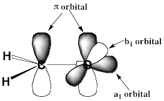
Figure 2.7. Bonding p and non-bonding oxygen-centered a1 and b1 MOs in formaldehyde.
The HF single determinant wave function for the neutral formaldehyde molecule is of the following form: |... pa pb a1a a1b b1a b1b| where the dots ... denote all of the other doubly-occupied MOs (i.e., the C and O 1s pairs, the C-O sigma bond pair, and the two C-H bond pairs). For the anion in which one adds an electron to the C-O p* orbital, the corresponding HF wave function is |... pa pb a1a a1b b1a b1b p*a|.
The difference between the correlation energy of the neutral and anion arise largely from two sources:
- The anion's wave function will contain double excitations in which one electron is excited from the p*a spin-orbital and another is excited from one of the other spin-orbitals (... pa pb a1a a1b b1a b1b). These contributions to the wave function, which do not occur in the neutral molecule's wave function because the p*a spin-orbital is absent, allow the p*a electron to avoid the other sixteen electrons. This class of double excitations (i.e., in which the excess electron is excited to a virtual orbital and another electron of the neutral molecule is also excited) produce much of the dispersion (i.e., van der Waals) interaction between the attached electron and those of the neutral molecule. In the example being considered, they produce the van der Waals interaction between the p*a electron and the other electrons.
- The neutral's wave function will possess certain terms that the anion's wave function does not. In particular, double excitations from any two of the spin-orbitals ...pa pb a1a a1b b1a b1b that appear in the neutral's HF determinant into the p*a spin-orbital and another (e.g, p*b, or some higher-energy virtual) orbital occur in the neutral but can not occur in the anion because the p*a spin-orbital is occupied in the anion. In other words, the fact that the anion has an electron in the p*a spin-orbital excludes the other electrons from using excitations into the p*a spin-orbital to form polarized orbital pairs and thus allow for their correlations.
It turns out that the combination of the above two differential electron correlation contributions makes the correlation contribution to the EA a significant quantity that essentially always must be addressed.
X. Reaction Paths
Another component of many electronic structure calculations is locating local minima and transition states on Born-Oppenheimer electronic energy surfaces. This is usually accomplished by using the derivatives of the electronic energy with respect to displacements of the anion's nuclear positions and searching for geometries at which the first derivatives vanish. The first derivatives gK= ∂E/∂XK are know as the gradients of the energy with respect, for example, to the Cartesian coordinate XK (e.g., the x, y, or z coordinate of one of the atoms in the anion). The second derivatives HK,L= ∂2E/∂XK ∂XL form elements of a 3Nx3N matrix (N being the number of atoms) called the Hessian matrix. At a local minimum (i.e., corresponding to a geometrically stable structure), all 3N elements of the gradient vector vanish and all but one of the eigenvalues of the Hessian matrix are non-negative. At a transition state, all elements of the gradient vanish, but one eigenvalue of the Hessian is negative. The eigenvector (containing elements {VK0}) of the Hessian's negative eigenvalue gives the components of the direction of the reaction path along each of the 3N {XK} coordinates.
Assuming one has the gradient available for an anion at some starting geometry whose Cartesian coordinates I will denote X0 = {X1, Xz, ... X3N}, one can attempt to find a local-minimum structure by making a series small displacements dXK (often called steps) in each of the coordinates proportional to, but in opposition to, the gradient gK along that direction
dXK = - a gK.
This step would be expected (i.e., using the first-derivative expansion of the energy) to yield an energy change
dE = SK dXK gK = - a SK |gK|2
that is negative. The size of the step (a2 SK |gK|2) can be controlled by choosing the parameter a. One cannot use too large a step length or one will no-doubt move so far that the linear approximation dE = SK dXK gK will no longer be valid. After altering each of the coordinates by dXK, one arrives at a new geometry XK + dXK. At this new geometry, one then recomputes the gradient vector and begins the above process anew, thereby generating a series of steps designed to find a local minimum. Once one has found a geometry at which all 3N elements gK vanish (to some specified accuracy), one stops. This strategy of stepping downhill (i.e., in opposition to the gradient vector) to search for a local minimum is indeed widely used and highly successful.
If one has both the gradient vector and Hessian matrix available, one can use a local quadratic approximation to predict the energy change accompanying a step dXK:
dE = SK gK dXK + ½ SK,L HK,L dXK dXL.
It is common when using this level of analysis to express the coordinate changes dXK in terms of the eigenvectors VKa of the Hessian matrix:
SL HK,L VLa = la VKa.
There are 3N eigenvalues (la; a = 1, 2, ... 3N) and 3N eigenvectors each having 3N components {VKa; a = 1, 2, ... 3N; K = 1, 2, ... 3N}. However, 6 (or 5 for a linear molecule) of these eigenvalues are zero and correspond to displacements describing translations (3) and rotations (3 or 2) of the system.
Because these eigenvectors form a complete set in this 3N-dimensional space, one has
Sa VKa VLa = dK,L.
So, the step dXK can be expressed as a sum of steps having magnitudes dVa along the VKa eigen-directions:
dXK= SL dK,L dXL = Sa VKa (SL VLa dXL) = Sa VKa dVa.
Substituting this into the quadratic expansion for dE allows one to express the energy change in terms of steps along these eigen-directions:
dE = Sa {ga dVa+ ½ la (dVa)2}
where
ga = SL VLa gL
is the component of the gradient along the ath eigen-direction. The components of the gradient along the 6 (or 5 for a linear molecule) eigen-directions corresponding to translations and rotations vanish. So, the sum Sa {ga dVa+ ½ la (dVa)2} can be restricted to 3N-6 (or 3N-5) directions.
The advantage to viewing dE in terms of contributions from components along the 3N-6 eigen-directions is that it allows one to separately analyze each of 3N-6 independent contributions. In this way, one can consider taking steps that are downhill (i.e. contributing a negative value to dE) along all directions or uphill along one direction and downhill along each of 3N-7 other independent directions. The former is used to find minima and the latter to locate transition states.
So, after one has computed the gradient and Hessian and found the 3N-6 non-zero eigenvalues and eigenvectors of the Hessian, one computes ga as above. To move downhill in all directions toward a local minimum, one then chooses each of the dVa steps to cause {ga dVa+ ½ la (dVa)2} to be negative. One can minimize {ga dVa+ ½ la (dVa)2} with respect to dVa to obtain an approximation to the optimal step
dVa = - ga/la.
This step is then predicted to contribute an amount {- ga2/la + ½ la (-ga/la)2} = -1/2 ga2/la to the energy change. For eigen-directions having positive la values, this step will decrease the energy, but for a direction having a negative la, the energy will increase. So, if one is seeking a minimum, one uses dVa = - ga/la only for those direction having positive la values, and one either takes no step along the direction having negative la or one reverses directions and chooses dVa = ga/la for this direction. On the other hand, when seeking a transition state, once one finds a geometry at which one eigen-direction has a negative la, one chooses dVa = - ga/la or move uphill along this direction [[67]].
Once one has found a local minimum, one can compute the harmonic vibrational energies at this minimum by forming the mass-weighted Hessian
MWHK,L = HK,L (mK mL)-1/2
dividing the elements of the Hessian computed in terms of Cartesian coordinates by the square roots of the masses mK and mL of the atoms associated with the Kth and Lth coordinates. To see why the mass-weighted Hessian's eigenvalues provide a route to vibrational frequencies, we consider the Hamiltonian for harmonic vibrational motions of the anion in the vicinity of this local minimum
H = SK,L ½ HK,L dXK dXL + ½ SK mK (ddXK/dt)2
expressed in Cartesian coordinates. This can be rewritten in terms of so-called mass-weighted coordinates
dMWXK = (mK)1/2 dXK
and the mass-weighted Hessian:
H = SK,L ½ MWHK,L dMWXK dMWXL + ½ SK (ddMWXK/dt)2 .
By transforming to the coordinates that diagonalize MWHK,L
dXK= Sa VKa dVa
this Hamiltonian reduces to
H = Sa {½ la(dVa)2 + ½ (dVa/dt)2}.
Recalling that 6 (or 5) of the la vanish, we see that this is the Hamiltonian for 3N-6 (or 3N-5) uncoupled harmonic oscillators having force constants la and having unit masses for all coordinates. As such, the harmonic vibrational frequencies are given by
wa = (la)1/2
thus showing that the eigenvalues of the mass-weighted Hessian provide the harmonic vibrational frequencies.
Once one finds a transition state, one can again form the mass-weighted Hessian at that geometry and find its 3N-6 (or 3N-5) non-zero eigenvalues. Of these, one will be negative and the others will be positive. The eigenvector {VK1} corresponding to the negative eigenvalue l1 has coordinates that point the way along the reaction path that starts at this transition state. The square roots of the 3N-7 (or 3N-6) other eigenvalues of the mass-weighted Hessian give the harmonic vibrational frequencies of the transition-state species' modes that lie perpendicular to the reaction path.
To trace out the reaction path starting at a transition state, one first finds the eigenvector {VK1}. One next takes a very small step along this direction (i.e, taking dXK = a VK1 with the a parameter being small). Because VK1 is an eigenvector of the mass-weighted Hessian, these step lengths are given in terms of the mass-weighted Cartesian coordinates defined earlier and thus they have units of m1/2distance. Taking the value of a positive moves one in one direction along the reaction path; choosing a negative moves one in the other direction. Both branches of the path need to be mapped out to join the transition state to both reactants (one path) and products (the other path). After taking a small step along this eigen-direction, one then recomputes the Hessian and gradient (n.b., the gradient vanishes at the transition state but not once begins to move along the reaction path) at the new geometry XK + dXK. At this geometry, one forms and finds the eigenvalues and eigen-directons of the mass-weighted Hessian and uses the local quadratic approximation
dE = Sa {ga dVa+ ½ la (dVa)2}
to guide one downhill. Along the eigen-direction corresponding to the negative eigenvalue l1, the gradient g1 will be non-zero while the components of the gradient along the other eigen-directions will be small (if one has taken a small initial step).
In effect, one is attempting to move down a streambed whose direction of flow initially lies along VK1 and perpendicular to which there are harmonic sidewalls ½ la (dVa)2. So, one generates a series of steps by
- moving (slowly, in small steps) downhill along the eigen-direction that begins at VK1and that continues along the eigen-direction having a significant gradient component ga,
- while minimizing the energy (to remain in the streambed's bottom) along the 3N-7 other eigen-directions (by taking steps dVa that minimize each {ga dVa+ ½ la (dVa)2}.
As one evolves downhill along this reaction path, one reaches a point at which the eigenvalue l1 of the mass-weighted Hessian along which the step displacement has its largest component changes sign from negative to positive. This signals that one has left the neighborhood of the transition state and one is approaching a local minimum. Continuing onward, one eventually reaches a point where the gradient's component along the step displacement vanishes as do all the other components. This is the local minimum that connects to the transition state at which the reaction path started. As mentioned above, one needs to also begin at the transition state and follow the other branch of the reaction path to be able to connect reactants, transition state, and products.
Of course, all that is said above assumes one has the gradient (and perhaps the Hessian) in hand, but it says nothing about how one obtains them. One of the major advances in ab initio electronic structure theory has been the derivation and computational implementations of equations for the gradient and Hessians. Professor Peter Pulay has been the major figure behind much of this development.

Peter Pulay, University of Arkansas
To evaluate the derivative of the Born-Oppenheimer energy E with respect to a Cartesian coordinate XK, one begins by writing an expression for E in terms of the electronic Hamiltonian H and wave function Y. For example, for Hartee-Fock or MCSCF wave functions,
E = <Y|H|Y>/<Y|Y>.
One then uses the chain rule to, for example, express the first derivative as
dE/dXK = {<Y|dH/dXK|Y>/<Y|Y> + <dY/dXK|H|Y>/<Y|Y> + <Y|H|dY/dXK >/<Y|Y>
- E < dY/dXK|Y>/<Y|Y> - E <Y| dY/dXK>/<Y|Y>}.
The wave function derivative terms dY/dXK involve ∂Y/∂Cj,m dCj,m/dXK and ∂Y/∂CJ dCJ/dXK for the HF and MCSCF cases. However, in these two cases the energy has been optimized with respect to the LCAO-MO and MCSCF coefficients, so the sum of the four terms on the right hand side of the expression for dE/dXK vanishes because this sum is equal to ∂E/∂Ci,m dCj,m/dXK or ∂E/∂CJ dCJ/dXK. This allows one to express the gradient in these cases in terms of the so-called Hellmann-Feynmann term
dE/dXK = <Y|dH/dXK|Y>/<Y|Y>.
In the Hamiltonian H, the only place the Cartesian coordinate XK appears is in the electron-nuclear potential involving the nucleus associated with coordinate XK. So,
dH/dXK = - Sj ZKe2 {(Xk-xj)/|RK-rj|3)
and thus the evaluation of dE/dXK requires that one evaluate the expectation value of this one-electron operator. Here, ZK is the charge of the nucleus associated with the coordinate XK, XK – xj is the distance along coordinate XK to the jth electron, and |RK – rj| is the total distance from this nucleus to the jth electron.
For the MPn, CI and CC cases, the evaluation of dE/dXK is more difficult because the expression used to obtain the electronic energy E in these cases has not been minimized with respect to both the Cj,m and CJ coefficients. As a result, one has to derive and implement so-called response equations that describe how these coefficients vary with XK. Nevertheless, these derivations have been carried out and so energy gradients can be evaluated even in the MPn, CI, and CC situations. It is beyond the scope of this text to go further into these matters, but there are excellent sources [[68]] for learning more about them.
XI. Summary
Let us summarize some of the most important things that one needs to keep in mind when studying anions using theoretical methods:
- Basis sets should be used that (i) are flexible in the valence region to allow for the different radial extents of the neutral and anion's orbitals, (ii) include polarization functions to allow for good treatment of electron correlations, and (iii) include extra diffuse functions if very weak (< 0.3 eV) electron binding is anticipated. For high precision, it is useful to carry out basis set extrapolations using results calculated with a range of basis sets (e.g., VDZ, VTZ, VQZ).
- Electron correlation should be included because there is substantial differential correlation energy in the EA. Correlation allows the electrons to avoid one another by forming polarized orbital pairs. There are many ways to handle electron correlation (e.g., CI, MPn, CC, DFT, MCSCF).
- Single determinant zeroth order wave functions may not be adequate if the anion or neutral's spin and space symmetry adapted wave function requires more than one determinant. Open-shell singlet wave functions are the most common examples for which a single determinant cannot be employed. In such cases, methods that assume dominance of a single determinant should be avoided.
- Most current DFT functionals display incorrect r-dependence at large-r, so their use, especially for weakly bound anions, can be problematic.
- The computational cost involved in various electronic structure calculations scales in a highly non-linear fashion with the size of the AO basis, so careful basis set choices must be made.
- Although it is not treated until Chapter 5 Section IV, special techniques need to be used when treating an anion whose electronic energy lies above that of its parent neutral. Such electronically metastable anions cannot straightforwardly be handled with conventional (i.e., MPn, HF, Koopmans' theorem, CC, CI, or MCSCF) methods without these special techniques also being utilized. If one tries to calculate the anion's energy using such conventional means, in most cases one will end up describing the neutral parent with a single excess electron far from it and with low or zero kinetic energy rather than the desired metastable anion. That is, one will obtain nonsensical results.
- There exist methods that allow one to compute the intensive EA directly rather than by computing separately the neutral and anion energies. Because the latter are extensive quantities, they are more susceptible to numerical imprecision as the system size grows in which cases these direct-calculation (e.g., EOM) methods are most useful.
- There are tools based upon the first and second derivatives of the Born-Oppenheimer energy with respect to atomic coordinates that allow one to trace out reaction paths connecting reactants, transition states, and products.
Chapter 3. Chemically Conventional Anions
I. What Makes these Anions Conventional?
In this Chapter, we will focus discussion on molecular anions that are electronically and geometrically stable (i.e., that do not undergo autodetachment or spontaneous fragmentation) and that form common building blocks in chemistry. All of these anions bind their excess electron(s) in valence orbitals, which is the primary reason I call them chemically conventional. However, their electron binding energies range from less than 0.1 eV (e.g., for H3C-and many other alkyl anions) through and beyond 3.9 eV (e.g., for NC-), so the accuracy required to evaluate their binding energies to within a given percent and the kind of atomic orbital basis sets needed to describe their valence orbitals vary substantially even within this family.
Most such anions are not especially difficult to prepare, control, and probe (by spectroscopy or reaction dynamics) in the laboratory using one or more of the techniques discussed in Chapter 1 of this text. The current state of the art in determining the electron binding energies of such anions either by experimental means or via quantum chemical calculation is reviewed in several places, so we will not spend a great deal of time doing so here. Several books and reviews provide the reader with a good overview of such anions. Massey's classic book [46] and Branscomb's [47] chapter treat many of the difficulties involved in making anions and studying them by photoelectron or photodetachment spectroscopy. The status of theoretical studies on such anions dates from Berry's review in 1969 [45], through Jordan's in 1978 [[69]], Simons' and Jordan's in 1987 [42], Kalcher's and Sax's in 1994 [43], Kalcher's in 1996 [[70]], to one in 2001 from the Schaefer and Ellison groups [14]. The latter review also contains an up-to-date tabulation of many atomic and molecular electron affinities obtained by a variety of experimental means as well as by some quantum chemical methods. The tabulations offered in the latter review represent the current state of the art and are the first source one should consult when faced with finding the electron affinity of an atom or molecule, especially one that holds its excess electron in a conventional valence orbital. The research group of Professor Carl Lineberger, in particular, has been involved in determining many of these electron affinities using spectroscopic methods.
Returning to the issue of conventional molecular anions, we first note that the same kind of atomic orbital basis sets (i.e., conventional core and valence, polarization, and conventional diffuse) can be used within Hartree-Fock, DFT, or correlated treatments of their electronic structure. Because they hold their excess electron(s) in valence orbitals, the extremely diffuse basis sets [50] used, for example, on Rydberg and dipole-bound anions need not be employed. However, because EAs are inherently small quantities (e.g., even the EA of a halogen atom is only ca. 3.5 eV), the electronic energies of the anion and neutral must be computed with high accuracy. This means that one usually must treat dynamical electron correlation at a reasonably high level. For these reasons, even the seemingly simple task of computing EAs of, for example, F, Cl, OH, SH, NO2, or CH2 involve significant computational challenges. Note that we did not list any multiply charged anions in this discussion of conventional anions. It turns out that such species, although (seemingly) familiar and common in the laboratory, involve very special challenges to their theoretical treatment that render them by no means conventional. Therefore, we treat multiply charged anions in a separate Chapter where we discuss the special tools needed to properly treat their electronic structures.
II. They May be Conventional, but They Involve Complexities
There are special issues that one must be aware of in studying all anions, including conventional valence-type anions. For example, the EAs of such species are often smaller than the bond strengths connecting the anion's constituent atoms. As a result, one must be prepared to consider electron detachment processes in addition to bond fragmentation whenever a significant amount of excess energy is present. This situation is not typical of neutrals and cations for which electron removal involves energy considerably in excess of bond dissociation energies.
An example is provided by the NH-(X 2P) → e- + NH(X,3S) process in which an electron can be ejected from the anion once it has enough vibrational energy to place it above the lowest vibrational level of the neutral NH. It turns out that even the v = 1 level of NH-lies high enough to allow this to happen because NH has a very small EA. The pertinent potential energy curves and state energies are illustrated qualitatively in Fig. 3.1.
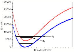
Figure 3.1. Anion (lower) and neutral (upper) potential energy surfaces illustrative of NH- and NH.
In this case, the electron binding energy is less than 0.5 eV, which is much smaller than the NH bond strength. Thus, as vibrational energy is deposited into NH- either by heating or by photon absorption, the electron-detachment channel opens far before the bond-fragmentation channel does. So, for example, in collisions of NH- with other molecules, one should not expect to first detect H- + N as the collision energy is increased; instead, one likely will observe NH + e-, but higher energies, H- + N and even e- + N + H could be expected.
Notice that the potential energy curve of the NH- anion does not intersect that of the NH neutral. This tells us that there is no N-H bond length R at which the anion's electronic energy lies above that of neutral NH. This, in turn, means that the NH- anion is not an electronically metastable species as, for example, N2- (X2Pg) is and as we will discuss in more detail in Chapter 5. So how then does the electronic energy of NH- become increased sufficiently to generate the (electronically) higher energy NH + e- state lying in the continuum?
The mechanism by which the NH- anion's excess electron is ejected involves coupling between the electronic and vibrational energies of the NH- anion. Specifically, so-called non-Born-Oppenheimer couplings give rise to this energy flow. These couplings involve derivatives of the electronic wave function Y with respect to a nuclear-motion coordinate Q and derivatives of the vibration-rotation wave function |v> with respect to this same coordinate: dY/dQ d|v>/dQ. That is, the vibrational mode loses energy (and momentum) as the electronic degree of freedom gains energy (and momentum). As a result, the rate of electron ejection is related to the derivative of the orbital out of which the electron is ejected with respect to the vibrational (or rotational) motion that is inducing the ejection. The author's research group has been involved in studying the rates of such non-adiabatic transitions in molecular anions over a long time period [[71]] in close collaboration with experimental groups who also study them [[72]] including those of Professors Carl Lineberger, John Brauman, and Torkild Andersen.
In the NH- case, the couplings that cause electron ejection involve how the 2pp orbital located on the nitrogen atom responds to vibrations and rotations of the N-H internuclear axis. In Fig. 3.2 these dynamical responses are illustrated.
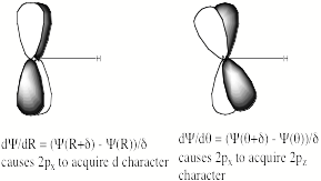
Figure 3.2. Orbital response of NH- 's 2pp orbital to (a) vibration of the N-H bond (left) and (b) rotation of the N-H bond (right).
For NH-, the non-bonding nitrogen 2pp orbital is modulated very little by vibration of the N-H bond (R) (i.e., dY/dR is small), so the resultant rate of vibration-induced electron ejection is small. On the other hand, if the rotational motion is excited to high J-levels, the angular couplings arising from the kind or rotation-induced orbital changes shown on the right side of Fig. 3.2 are more capable of producing electron ejection.
In contrast to the NH- case, when the H2C-C torsional vibration is excited in an enolate anion R2-C-CH2-O-, the rate of electron ejection can be much larger. In Fig. 3.3 the energy curves for a typical enolate anion (lower) and its daughter neutral radical (upper) are shown as functions of the torsion angle. Also in this figure is shown the orbital out of which an electron is ejected as the torsional motion evolves.
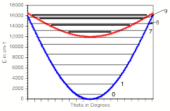
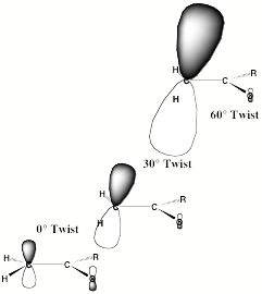
Figure 3.3. Anion (lower) and neutral (upper) potential energies for a typical enolate along with the evolution of the HOMO out of which an electron is ejected as a function of the torsion angle.
For such cases, the anion's HOMO is highly delocalized (in this case over both carbon atoms and the oxygen atom) when the anion is near its equilibrium geometry. However, as the torsional motion is excited and the corresponding angle deviates significantly from it equilibrium value, the HOMO's delocalization is interrupted. As a result, this orbital's energy increases, causing the anion-to-neutral energy gap to shrink as indicated in the top part of Fig. 3.3. Moreover, this orbital becomes more highly localized and its radial size grows (because its binding energy decreased). So, for enolates, the orbital from which an electron is ejected is very strongly modified by vibrational motion (especially the torsional mode), so the rate of ejection can be large.
The research groups of Professors John Brauman and Jack Beauchamp have studied such processes by using infrared lasers to vibrationally excite anions
and then detecting the electron-loss process. An example from the Brauman group [[73]] is shown in Fig. 3.4.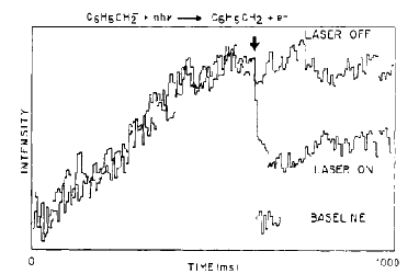
Figure 3.4. Intensity of benzyl anions in an ICR cell as a function of time after IR laser radiation is turned on.
Here we see experimental data in which benzyl anions are generated within an ICR cell (during the rise in the signal in Fig. 3.4) until a saturated signal is reached. If IR laser radiation (2 J cm-2 fluence at 948 cm-1) is exposed to the benzyl anions over a known time duration, the anion intensity drops as shown in Fig. 3.4. What happens as the IR photons are absorbed is much like we discussed for the enolate case described in Fig. 3.3. No single IR photon has enough energy to detach an electron from a benzyl anion whose electron binding energy is ca. 0.8 eV. Many IR photons must be absorbed until the torsional motion of the –CH2 group is sufficiently excited to disrupt the delocalization of the attached electron's p orbital and render detachment possible as in Fig. 3.3.
The ion ICR signal before I0 and after I laser excitation can be used to evaluate the cross-section s for IR-induced electron detachment of enolate anions by
ln (I/I0) = - s F
where F is the number of IR photons per cm2 per second striking the sample (this can be computed knowing the fluence in J cm-2 and the photon energy). For the benzyl anion, the workers of ref. 73 determined this cross-section to be s = 3.7 x10⁻²¹ cm2. They verified that the loss of anion signal was indeed due to electron detachment rather than ion fragmentation by inserting CCl4 into the ICR cell and observing that Cl- ions formed in proportion to benzyl anion loss (the CCl4 scavanges the ejected electrons).
An example of analogous IR multi-photon (in the case just discussed and in this case, more than one IR photon must be absorbed to eject an electron) electron detachment from the Beauchamp group [[74]] generated the data shown in Fig. 3.5.
 Figure 3.5. Loss in allyl anion signal after irradiation with IR light as a function
of the irradiation time.
Figure 3.5. Loss in allyl anion signal after irradiation with IR light as a function
of the irradiation time.
In this experiment, allyl anions were formed in two reactions- one using proton abstraction by NH3 and another using NF3 to remove TMS as suggested in Fig. 3.5. The data were interpreted to mean that the allyl anions formed in either reaction were internally (i.e., vibrationally) excited and only the hot ions in the sample underwent IR-induced electron detachment during the ca. 200 ms maximum duration of the IR excitation. The remaining fraction of the allyl anions were colder and would thus undergo much slower electron loss because they required more IR photons to allow them to reach the detachment threshold. As in the benzyl anion and enolate anion cases discussed earlier, once sufficient IR energy has been absorbed, the torsional motion of the –CH2 group disrupts the delocalization of the p orbitals thus making electron detachment possible.
In all such non-adiabatic electron-ejection processes, the rate of ejection is governed not only by how strongly the HOMO is modulated by the vibration (or rotation), but also by Franck-Condon-like factors [71]. These factors do not involve the overlap <vi|vf> of the anion and neutral vibrational states. Rather, they involve the overlap of the neutral's vibrational state vf with the derivative of the anion's vibrational state with respect to the vibrational coordinate (Q) that promotes the detachment <dvi/dQ|vf>. Because the electron ejection requires energy input, the vibrational mode that promotes the ejection must contribute some energy as a result of which it is left with less energy as it undergoes a change in quantum number. This change in quantum number is related to why the derivative dvi/dQ occurs instead of vi .
For the NH- example shown in Fig. 3.1, a vi =1 → vf = 0 change takes place. However, for the enolate example depicted in Fig. 3.3, the lowest transition that is energetically possible is a vi = 7 → vf = 0 transition. As a result, the Franck-Condon-like factors (i.e., the squares of <dv0/dQ|v7>, which are very small for this case) reduce the enolate's electron ejection rate below what the HOMO orbital's modulation would suggest, but have little such affect for NH- (because the derivative of the NH- anion's v = 1 vibrational wave function overlaps well with the v = 0 function of NH so <dvi/dQ|vf> is large).
Another example of how conventional anions can display unexpected behavior is taken from a study by Professor Kwang Kim's lab involving the atomic I- ion surrounded by six water molecules. In Fig. 3.6 we show, for each of four low-energy structures of the I-(H2O)6 cluster, the highest occupied molecular orbital [[75]] that is essentially an Iodine p orbital as well as the two lowest-lying excited orbitals (labeled LUMO1 and LUMO2).
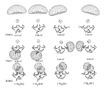 Figure 3.6. Highest occupied and two lowest-energy excited orbitals for four low-energy
isomers of I- with six water (W) molecules solvating it.
Figure 3.6. Highest occupied and two lowest-energy excited orbitals for four low-energy
isomers of I- with six water (W) molecules solvating it.
Two features in Fig. 3.6 might be somewhat surprising. First, it appers that the I- ion prefers to remain in a surface-solvated environment rather than to be more symmetrically surrounded by the six water molecules. Actually, this behavior is observed in other anions and derives from a competition between the energy and entropy costs needed to break hydrogen bonds connecting the water molecules as a network and the strength of the water-anion attractive potential (that includes electrostatic attraction as well as dipole-polarization interaction). The second perhaps surprising attribute of the orbital pictures shown in Fig. 3.6 is the fact that the excited orbitals do not seem to belong to the I- anion; instead, LUMO1 seems to be bound to the water cluster and LUMO2 resides outside the cluster and away from the I-. We will have more to say about what is called charge-transfer-to-solvent electronic excitations later in Chapter 6, so I will not pursue the nature of these excited orbitals further at this time, but the orbitals shown in Fig. 3.6 suggest that something unusual and exciting arises in such solvated-anion cases.
The above examples serve to show that even what we usually consider chemically conventional anions can display behavior that is not common in neutrals and cations. Some of the unusual behavior of anions is a result of the fact that EAs are usually smaller than bond dissociation energies, so electron detachment can be the first process that becomes possible as the anion's internal vibrational and/or rotational energy increases. We will have more to say about such detachment processes in the next Chapter when we discuss so-called dipole-bound anions. For such anions, it is the rotation of the molecular framework that can most efficiently promote electron ejection because it is this motion that couples most strongly to modulate the binding energy of the anion's HOMO.
III. Common Multiply Charged Anions are Not Conventional
Before closing this Chapter, let me point of several anions that we have not included here but that one might have expected us to discuss. Multiply charged anions such as SO42-, CO32-, and PO43- are ubiquitous in chemistry, but it turns out they are not stable with respect to autodetachment as isolated species. That is, gas-phase sulfate, phosphate, and carbonate (as well as numerous other small multiply charged anions) are not as conventional as we might believe. In fact, they exist as electronically stable species only when they are surrounded by stabilizing solvent molecules or within crystal lattices where counter cations stabilize them. For these reasons, we discuss these species in Chapter 5, which specifically deals with multiply charged anions and the extra issue of metastability that they involve.
Of course, there are multiply charged anions that are electronically stable, but these too I decided to include in Chapter 5. Examples of such stable multiply charged anions include those with two anion sites separated spatially by linker groups (e.g., dicarboxylates such as -O2C-(CH2)n-CO2-) as well as more exotic anions (e.g., TeF82- or MgF42-) that derive stability by delocalizing their excess charges over multiple ligands to reduce the internal Coulomb repulsions among the excess charges. An example that was studied by Professor Paul Kebarle's group [[76]] is the C5O52- dianion shown in Fig. 3.7.
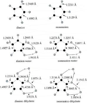
Figure 3.7. Structures of the C5O52- dianion as well as its mono-anion and their complexes with one and two water molecules.
This dianion is stable because its oxygen centers have high intrinsic electron binding power and because the two excess charges are delocalized over five carbon-oxygen units.
As I said, we decided to include most of our discussion of multiply charged anions in Chapter 5, so let us now move on to examine the next family of anions, those that result from binding an excess electron electrostatically rather than in a conventional orbital.
Chapter 4. Multipole-Bound Anions
I. Electrostatic Attractions
In this Chapter, we will deal with molecular anions in which the extra electron is bound to a large extent by the long-range electrostatic potential of the underlying neutral molecule rather than by shorter-range valence potentials. In such anions, the excess electron does not reside in a conventional valence orbital but in an orbital whose size, shape, and binding energy is governed to a large extent by the long-range electrostatic potential of the molecule.
When the dominant such interaction is the electron-dipole potential (-m cosq e2/r2), one speaks of dipole-bound anions such as in the cases of HCN-, -H3C-CN and the others whose dipole-binding orbitals are shown in Fig. 4.1. Notice that the species binding the excess electron may be an intact molecule such as HCN, but it can also be a complex or cluster of molecules bound to one another by van derWaals or hydrogen bonding forces such as in anions of the small clusters (HF)2 and (H2O)2.
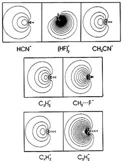
Figure 4.1. Dipole bound orbitals for a variety of anions. Notice that these orbitals are so large that it is difficult to show the molecular framework in the same figure.
Even larger biological molecules such as some DNA bases can bind an electron by way of their dipole potentials. In Fig. 4.2 the orbitals occupied by a dipole-bound electron in uracil and in a complex involving uracil and a water molecule [[77]] from Professor Ludwik Adamowicz's group are shown. The latter example illustrates that the size and shape of the dipole-bound orbital can depend significantly on where neighboring solvent molecules reside. This happens both because the solvent molecule (in this case, water) possesses a significant dipole of its own and because the solvent molecule may reside in a region of space where the solute's own dipole-bound orbital would have large amplitude thus blocking the ability of the solute to bind the electron in this location.
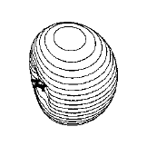
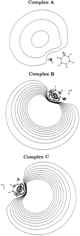
Figure 4.2. Dipole-bound orbitals of uracil base (left) and of uracil-water complex (right) at three different geometries.
In Fig. 4.3 we see another complex consisting of indole and a water molecule along with the dipole-bound orbital associated with the lowest-energy structure of this complex. The groups of Professors Charles Desfrançois and Jean Pierre Schermann teamed up with Professor Ludwik Adamowicz's group to perform this study [[78]].
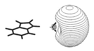
Figure 4.3. Lowest-energy structure of uracil-water complex and the dipole-binding orbital an electron attaches to to form the anion.
As we discussed in Chapter 1, the Schermann-Desfrançois team uses Rydberg atoms in various quantum states (n) to effect an electron transfer to the dipolar molecule thus forming the dipole-bound anion. In Fig. 4.4 we show plots of the intensity of dipole-bound anions formed for indole, indole(H2O), and indole(H2O2 as functions of the atom's Rydberg quantum number n (in this case, they used Xe atoms in f-orbital excited states).
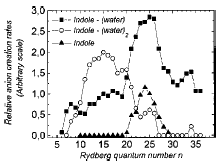
Figure 4.4. Yields of dipole-bound anions as functions of Rydberg quantum number n.
For the indole molecule, we note that there is a peak near n = 24 in the yield of anions formed. Using a theoretical model developed earlier by Professor Desfrançois [[79]], these workers could approximate the electron binding energy of the dipole-bound indole by
EA(eV) = 23 nmax-2.8,
where nmax is the value of the Ryberg quantum number at which maximum anion formation occurs (nmax = 24 for indole, so EA = 0.003 eV). For the indole(H2O)2 complex, nmax =15, so the dipole-bound anion is predicted to have an electron affinity of EA = 0.01 eV. As can be seen in Fig. 4.4, for the indole(H2O) system, there are two or more peaks in the anion-yield plot. This was interpreted in ref. 78 to be due to more than one indole(H2O) structure being present in the experimental sample, so anions having more than one EA are formed.
Many of the molecules that form these dipole-bound anions are closed-shell species (e.g., H3C-CN, uracil, H-CN or (HF)2) that have no low-energy vacant valence orbitals into which the electron can enter. Thus, the lowest-energy anion states that can be formed in such cases are the anions in which the electron is bound to a region of space dictated by the attraction of the electron-dipole potential rather than by the availability of an empty or half-filled valence orbital.
When these species are formed from clusters of polar molecules, such as the (HF)3- anion shown in Fig. 4.5, there usually are several structures that are local minima on the ground-state electronic energy surface. Some of these structures are of the dipole-bound kind (labeled dbe) having the molecular constituents arranged to maximize the total dipole moment while others are of the solvated-electron type (labeled se) in which the electron is surrounded by molecules whose dipole moments are directed inward. Of course, the latter structure is very energetically unfavorable in the absence of the excess electron. Hence, when photoelectron spectroscopy experiments are carried out on such solvated-electron structures, one encounters very large geomety changes and thus very unfavorable Franck-Condon factors. This, in turn, makes it extremely difficult if not impossible to determine adiabatic electron binding energies for such states.
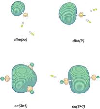
Figure 4.5. Four local-minimum structures of the (HF)3- anion that differ in how the dipole moments of the the HF molecules are oriented.
When one is faced with carrying out, for example, spectroscopic studies on such species, it is often very difficult to know which of the structures are present in the laboratory sample and which spectroscopic features correspond to which isomer. For example, even if selected on the basis of charge-to-mass ratio using a mass spectrometer, a sample may contain all four, or three, or two or only one of the (HF)3- species shown in Fig. 4.5. In such cases, it is very useful to have available good theoretical calculations of the relative energies (and entropies so that free energies can be estimated), vibrational frequencies, and electron binding energies of all isomers so that the experimental findings can be more readily interpreted. Of course, it may also be possible to use preparative techniques or experimental conditions such as temperature that favor forming some isomers over others to further simplify matters.
There are species that have both valence-bound and dipole-bound states. For example, deprotonated acetonitrile H2C-CN- is an anion in whose ground state the excess electron resides in a valence 2pp orbital on the carbon atom of the H2C- group as shown in Fig. 4.6.
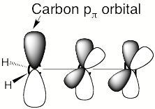
Figure 4.6 Half-filled carbon pp orbital in the H2C-CN- anion.
As such, it is a valence-bound anion. However, upon excitation of an electron from this pp valence orbital to the lowest excited state, the H2C-CN- anion holds its excess electron in a dipole-bound orbital that is localized to the left of the two hydrogen atoms in the H2C-CN framework and thus near the positive end of this molecule's dipole moment.
The above examples introduced the idea that a molecule with no empty or half-filled valence orbitals available to bind an electron might still bind an electron using its dipole potential. To appreciate the nature of such electron binding, it helps to consider the types of potentials an electron experiences as it approaches a polar neutral molecule. Because the molecule is neutral, there exists no long-range Coulomb potential (of the form –qe2/r). The potential that has the longest range (i.e., the smallest inverse power of the distance r between the electron and the molecule) is the charge-dipole potential
Vdipole = - mecosq/r2.
Here, m is the dipole moment of the molecule and q is the angle between the molecule's dipole vector m and the electron's position vector r. Of course, there are other potentials whose dependence on r is different. For example, the charge-induced-dipole potential is
Vpolariz. = -a• •rr e2/2r6,
where a is the polarizability tensor of the molecule and again r is the position vector of the attached electron, and the charge-quadrupole potential has the form
Vquad = -e Q• •(3rr-r21)/3r5
where Q is the quadrupole tensor of the molecule and 1 is the unit tensor.
For any molecule with a non-vanishing dipole moment m, it is the charge-dipole potential that must be treated first when considering weakly bound electrons because this potential has the longest range (i.e., dies off with the smallest power of 1/r). If |m| = 0, one must consider the effects of the charge-quadrupole potential, and, if Q vanishes, one has to look at even shorter-range potentials as possible electron binding sources. Let us first consider what is known about dipole binding.
A. The Point and Fixed Finite Dipole Models
Over fifty years ago, Fermi and Teller [[80]] and Wightman [[81]] carried out analyses of the Schrödinger equation
(- h2/2me∇2 - me cosq/r2) Y= E Y
describing the motion of a single electron of mass me in the presence of a purely attractive charge-dipole potential. Actually, Fermi and Teller were not studying electron-molecule interactions but attachment of negative p and m mesons to hydrogen atoms, a problem that has the same Schrödinger equation as the electron-dipole problem we are discussing. More recently, the group of Professor Sabre Kais [[82]] showed how dimensional scaling methods can be used to address this problem and Professor Ken Jordan's group provided a nice overview [[83]] of the status of dipole-bound anions following another recent review by Professors Gutowski, Jordan, and Skurski [[84]].
The Schrödinger equation containing only the kinetic and charge-dipole potential is commonly referred to as the point dipole (PD) model equation because it contains no compensating repulsive potential at small-r. The early workers noted above showed that if the magnitude of the dipole moment m exceeded 1.625 Debyes (or 0.693 ea0, where a0 is the Bohr radius 0.529 Å and e is the charge of the electron), the dipole potential is strong enough to support bound states of s symmetry (i.e., having azimuthal angle dependence exp(ilf) with l = 0) . On the other hand, if m < 1.625 D, no s bound states can exist. Even higher critical dipole moments are required to bind p and higher-l states (e.g., 9.6375 D for p states and 24.218 D for d states). However, it turns out that the PD model produces an infinite binding energy for its bound states, so it is quite unreasonable in this aspect, but it suggests that there may be a critical strength to the dipole potential that is needed before an electron can be bound, and this idea of a critical dipole moment survives even when more sophisicated potentials are employed.
Later, Crawford [[85]] and Dalgarno [[86]] and Byers-Brown and Roberts [[87]] among others considered both the point dipole and the fixed finite dipole (FFD) models for one electron moving in the presence of a pure dipole potential. The former model was discussed above; the latter considers two charges q and -qseparated by a distance R which define a dipole moment of magnitude m = qR as shown in Fig. 4.7.
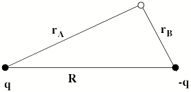 Figure 4.7. Parameters of the Fixed Finite Dipole Model
The Schrödinger equation for an electron moving under attraction to the center (A) of charge q and repulsion from center B of charge –q
(-h2 /2me ∇2 + e q [-1/rA + 1/rB]) Y = E Y
can be rewritten in terms of confocal elliptical coordinates
r = (rA + rB)/R , n = (rA –rB)/R
and the azimuthal angle f. Doing so is appropriate because of the f-independence of the potential and yields
{∂/∂r[r2-1] ∂/∂r + ∂/∂n{1-n2] ∂/∂n +[1/(r2-1) + 1/(1-n2)] ∂2/∂f2
-(er2 -en2 +bn)}Y = E Y.
Here e = - meR2E/2h2, and b = 2meRqe/h2 are variables that contain the energy E and the dipole moment Rq, respectively. The dependence of y on r and n can be separated using Y = u(r) n(n) exp(ilf). Doing so produces separate equations for the u and v functions:
∂/∂r[r2-1]∂u/∂r -er2u - ul2/(r2-1) + Bu = 0
∂/∂n{1-n2]∂n/∂n +(en2 - bn)n + nl2/(1-n2) –Bn = 0,
where B is the separation constant arising when the two-dimensional partial differential equation is reduced to two one-dimensional equations.
It is important to notice that the variable e depends on both the energy E and the dipole's length variable R. In contrast, the variable b is independent of E and depends only on the dipole's magnitude m = q R (i.e., only on the product of q and R). Byers-Brown and Roberts noted that these dependences of e and b allow one to conclude that requiring solutions u and n to exist having vanishingly small positive e would place demands on the magnitude of b and thus only on the magnitude of m, not the sizes of R and q separately. In other words, for the FFD model, the conditions for critical electron binding were shown to depend not on R and q separately, but only on the product q R = m, which is the dipole moment.
Moreover, as discussed in the review by Turner [[88]], several groups found that the value of m for which the FFD model barely binds an electron in a s state is exactly the same 1.625 D as the critical dipole moment for the PD model. The critical moments for binding p and d states in the FFD model are also the same as in the PD model. The main difference between the predictions of the two models lies in the binding energies they predict for m > 1.625 D. For m greater than the critical values, the PD model gives infinite binding energy whereas the FFD model gives finite binding.
Furthermore, it was shown that, even if one adds to the PD or FFD potential any short-range (decaying more rapidly than 1/r2) repulsive potential, exactly the same minimum values of m are needed to critically bind an electron. However, when such a repulsive potential is added, the binding energy predicted in the PD case is no longer infinite, and the binding energies now depend not only on m but also on the nature of the short-range repulsive potential for both the PD and FFD cases.
What do these results have to do with binding electrons to real molecules that contain other electrons and molecules that might be rotating or vibrating? The answer is that, although the PD and FFD models suggest the existence of a critical dipole moment above which electron binding will occur, the quantitative predictions of these models do not fit real molecules very well. As noted above, the pure PD model predicts that once m exceeds 1.625 D, an electron will bind in a s state and the binding energy of this electron will be infinite! Clearly this prediction is incorrect since an infinite binding is unphysical and because one expects the binding energy to depend on the magnitude of the dipole. For m > 1.625 D, the FFD model predicts finite binding, but the binding energies it generates tend to be considerably larger than for real molecules having the same dipole moment. For example, if one uses the known dipole moment and bond length of LiF to define partial charges q = m/R and then employs the FFD model, one obtains too large an electron binding energy for LiF-.
In addition, Professor Oakley Crawford showed [[89]] that, if one allowed the nuclei to also rotate, the dipole-bound states' energies would be destabilized as a result of which the critical dipole moment needed to bind an electron depends on the rotational energy content of the system. One way to appreciate this observation is to note that the rotational average of the dipole potential is zero
![]() .
.
If the rotational motion occurs on a shorter time scale than the movement of the dipole-bound electron, the electron experiences the rotationally averaged potential which vanishes and thus is no longer capable of binding the electron. In practice, one finds that once the energy spacing between successive rotational levels exceeds the binding energy of the dipole-bound electron, the anion will become unstable with respect to auto-detachment because the dipole potential is attenuated by the rotational motions.
Although the PD and FFD models are highly suggestive of what to expect for electrons binding to real molecules, an experimental chemist wants to know how large m must be before significant electron binding (i.e., large enough to render the anion stable enough to be examined and to be within the range of experimental resolution) will occur, but neither model can do this very accurately. For example, Turner shows [88] that for m = 1.696 D, the FFD model predicts a binding energy of 10-18 eV. However, to achieve a binding energy of 1 cm-1 (which is about as small as could be experimentally probed), the FFD model suggests one needs m > 2 D. It is the latter value that would be of more experimental relevance if the FFD model's predictions were accurate enough to be trusted.
Another example of the limitation of the models is provided by the KH- anion at its equilibrium bond length (2.38 Å) where its dipole moment is 9.465 D. It turns out that the LiH- anion stretched beyond its own equilibrium bond length to R = 3.2 Å has the same dipole moment, m = 9.465 D. Because these species have the same m values, the FFD model suggests they should have binding energies (E) whose ratio is the square of the inverse ratio of their bond lengths. This relationship follows because the e parameter of this model is proportional to ER2, and it is e that is uniquely determined by m. The ratio of these two anions' binding energies is 0.35 eV/0.90 eV = 0.39, but the ratio of their bond lengths squared is (2.38/3.2)2 = 0.55. So, again, we see that the quantitative predictions of the FFD model are not very good.
What is wrong with the PD and FFD models that limits their applicability to realistic molecular systems? Professor Ken Jordan's group has done as much theoretical work as anyone in recent years to carefully probe the electronic structures of dipole-bound anions. They bridged the gap between the above PD and FFD models and more realistic descriptions. They also recently invented a clever, accurate, and very efficient way, based on the Drude model [[90]] used to treat dispersion (i.e., van der Waals) interactions that relate to the correlation of the dipole anion's excess electron with the underlying neutral's other electrons. Earlier workers had shown [[91]] such dispersive interactions between the weakly dipole-bound electron and the remaining electrons to be important to take into consideration.
While discussing models for the electron-molecule interaction potential, it is important to note a model that Professor Charles Desfrançois has developed [[92]] and applied very successfully to a wide range of electron-molecule complexes. This model allows one to study dipole-bound electrons as well as systems in which the electron is bound primarily by the electron-quadrupole or electron-polarization potential. It contains both attractive electrostatic potentials (e.g., charge-dipole, polarization, charge-quadrupole, etc.) an valence repulsion potentials, so it is capable of predicting electron affinities to reasonable accuracy.
Following up on the FFD model, Jordan and Luken [[93]] examined a generalization of the fixed finite dipole model in which one center has charge Z+q and the other center has charge –q, and the former center is surrounded by an electron distribution containing Z electrons. Foe example, one might model LiCl by one point charge 2+q and another –q separated by a distance R with two 1s electrons centered on the center of charge 2+q. The two 1s electrons' influence on the extra (dipole-bound) electron was approximated in the Jordan work in terms of Coulomb and exchange potentials
Vcore = Sp=1,Z (Jp – Kp).
These potentials, in turn, were expressed in terms of orbitals {fj j = 1, Z} obtained by solving the Hartree-Fock (HF) equations for the Z electrons in the presence of the two centers of charge Z+q and –q. Results showed that this modified FFD model could produce electron binding energies more accurately than could the original model. This therefore suggests that the primary deficiencies of the simple PD and FFD models are that:
- they ignore Coulomb and exchange repulsion produced by inner-shell electrons;
- they ignore orthogonality of the extra electron's orbital to those of the other electrons in the molecule (this causes the extra electron's orbital to not have the proper nodal structure);
- they ignore the indistinguishability of the electrons and thus the antisymmetry of the many-electron wave function within which the extra electron resides.
So, does this mean that the critical dipole moment suggested by the PD and FFD models is wrong? Not really! It is true that any non-rotating molecule with m > 1.625 D and any number of inner-shell electrons (i.e., any short-range repulsion) will bind an electron. However, the binding energy may be so small as to be experimentally irrelevant and certainly will depend on the nature of the inner-shell repulsions. In contrast, the modified FFD model discussed immediately above gives more useful approximations to the binding energies of real molecules. So, when one considers real molecules and the possibility of their binding an electron via dipole binding, one must consider
- the magnitude of the molecule's dipole moment (the larger this moment, the stronger the binding is likely to be), and
- the number and radial extent of the inner-shell orbitals whose Coulomb and exchange repulsions act to destabilize the excess electron (the more such orbitals exist near the positive end of the dipole, the weaker the binding).
As a result of these two competing factors, there really is no unique critical value of the dipole moment that will guarantee electron binding to a specified extent (e.g., to 1 cm-1). Nevertheless, for molecules comprised of first-row atoms (this relates to the number and sizes of their inner-shell orbitals), dipole moments in the 2.5 Debye range seem to be required before electron binding of a few cm-1 is observed. It should also be mentioned that although excited states can exist for dipole-bound species, it is rare to observe such states because their binding energies are much smaller than that of the ground state, which itself is usually a very small energy.
B. Binding to Real Molecules
There have been many theoretical and experimental studies of electrons bound to polar molecules in which the binding is ascribed primarily to the charge-dipole attractive potential. Recent reviews [[94]] offer excellent insight into the current state of affairs of the theoretical studies most of which have been carried out in the laboratories of Drs. Jordan [[93], [95]-[99]], Adamowicz [[100]-[117]], Chipman [[118]], Bartlett [[119]-[121]], Gutowski and Skurski [[98],[99],[122]-[130]], Schermann and Desfrançois [[131],[132]], and the author [[94],[95],[98],[99],[122]-[130] ,[133],[134]].
Much of the early experimental work on dipole-bound anions was produced in the Brauman [[135]-[143]], Lineberger [[143]-[150]], Schermann and Desfrançois [[151]-[164]], Compton [[158],[165],[166]] and Bowen [[167]-[171]] laboratories. More recently, Mark Johnson's group [[172]-[176]] has also generated a substantial body of data on such anions, and many other experimental and theoretical groups are joining these exciting studies.
For example, Professor Paul Burrow's group and collaborators have recently suggested [[177]] that dipole-bound states of uracil and thymine may act as doorway states for inducing bond cleavage in these DNA bases. In Fig. 4.8, we see uracil's dipole-bound orbital in two depictions as well as the N-H s* orbital. The idea put forth by Burrow et al is that an electron can initially be captured into the dipole-bound state after which stretching of the N-H bond causes the s* state to drop to lower energy. As the s* state drops in energy, it eventually couples with the dipole-bound state (they are of the same symmetry), an avoided crossing of these two states occurs, and the electron migrates into the s* orbital thus cleaving the N-H bond.
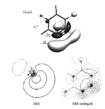
Figure 4.8. N-H s* orbital (top) and dipole-bound orbital (bottom) for uracil anion.
In nearly all of the studies of dipole binding discussed above, there is good reason to believe that the binding is due significantly to the dipole potential, but in no case can it be shown that the resultant anions are purely dipole-bound. Let us illustrate by examining a few anions that have been termed dipole-bound. The H3C-CN molecule has a dipole moment of 4.34 D and has been shown to form an anion with an electron binding energy of ca. 108 cm-1. Calculations show that the excess electron occupies an orbital localized on the positive end of this dipole within the H3C- group's pocket of three C-H bonds and rather distant from the underlying molecule's valence orbitals as shown in Fig. 4.9.
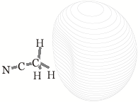
Figure 4.9. Orbital in which the excess electron resides in H3C-CN-.
Clearly, CH3CN has no vacant or half-filled valence orbitals that could attach the excess electron (its CN p* orbital is significantly higher in energy and, in fact, produces a metastable anion when occupied), so it is quite appropriate to call its anion dipole-bound. However, not all molecules having this dipole moment bind an electron to the same extent; for example, H2CCC also has a dipole moment of 4.34 D but binds by 173 cm-1 [[178]]. So, in reality the binding energy is determined not only by m but also by the nature of the molecule's other occupied orbitals as reflected in their Coulomb and exchange potentials.
Moreover, when one examines the contributions to the electron binding energy of the H3C-CN- anion, one finds that the electron-dipole attraction (plus other charge-multipole interactions) combined with the Coulomb and exchange interactions involving the excess electron do not reproduce the full electron binding energy. In fact, 57 cm-1 or 53 % of the binding arises from the dispersion interaction [98] between the excess electron and the other electrons of the neutral H3C-CN molecule. Such dispersion contributions have been found to be substantial in many dipole-bound anions. Hence, it is not correct to think of these species as being entirely dipole-bound although the charge-dipole potential is the effect that attracts the excess electron at the longest range.
Let's consider another example- that of acetaldehyde enolate [143] H-COCH2-, which has a valence-bound ground state and a dipole-bound excited state. In the ground valence-bound state, the excess electron occupies a delocalized orbital of p symmetry that is delocalized over the oxygen and the two carbon centers. In the excited state, an electron is promoted from this p orbital into an orbital that is bound primarily by the underlying radical's dipole potential. However, again the binding energy of this dipole-bound state is not entirely determined by the radical's dipole moment and the Coulomb and exchange repulsions of the other electrons. Dispersion interactions between the excess electron and the others are important, so again, the anion is not entirely dipole-bound. This example teaches another lesson- that even species such as the H2C-CHO radical that has a half-filled valence orbital and thus has a valence-bound anion can also form dipole-bound states if their dipole moments are large enough. That is, the fact that a species forms a valence-bound anion does not preclude it from also forming a dipole-bound state.
A more extreme example of the roles played by shorter-range potentials is offered when one considers anion states of alkali halides or alkali hydrides such as LiF-, NaH-, or the alkaline earth analogs such as BeO- or MgO-. For example, in neutral LiF, the bonding at the equilibrium internuclear distance is very ionic. Hence, one can view the neutral as a closed-shell F- anion sitting next to a closed-shell Li+ cation, although, of course, the electron densities of these two ions are polarized by their neighbor counter-ion. Undoubtedly, at very long distances from the LiF nuclei, the excess electron is attracted primarily by its dipole interaction with the Li+F-. However, in regions of space closer to the Li and F centers, the excess electron experiences both the repulsive Coulomb and exchange interactions mentioned earlier as well as valence-range attractive interactions when it is near the Li+ center, which has empty 2s and 2p orbitals. As a result, the excess electron feels the dipole potential at long range but a potential more like that experienced by a Li 2s electron polarized by a nearby F- ion at shorter range. So, in such cases, shorter-range valence potentials combine with the long-range dipole potential to bind the excess electron by a considerable amount. So, it is not appropriate to call ions such as LiF- purely dipole-bound although the dipole potential certainly contributes considerably to the binding.
In my opinion, calling an anion state dipole-bound reflects the fact that the state is electronically stable primarily due to the long-range attractive - me cosq/r2 potential, which produces an orbital localized primarily on the positive side of the molecular dipole and outside the range of the valence orbitals. This orbital, of course, also experiences shorter-range valence attractive and repulsive potentials and has dispersion interactions with the other electrons, all of which contribute to the total binding energy. So, I would categorize –HCN and –H3C-CN as dipole bound (albeit with considerable contributions to the binding arising from dispersion) and I would term the alkali halide anions as dipole bound with very substantial contributions from valence-range attractive potentials as well.
Another difficulty surrounding using the terminology of dipole-binding can be illustrated by considering the zwitterionic tautomer of, for example, a molecule containing a carboxylic acid and and amine group separated by a distance R as in HOOC- (CH2)n-NH2. Certainly (at a fully extended geometry) –OOC-(CH2)n-NH3+ has a huge dipole moment, so it is tempting to refer to the species obtained by adding an electron to the protonated amine site (i.e., –OOC-(CH2)n-NH3) as dipole-bound. However, at least in my opinion, this would be an incorrect use of the term dipole-bound; rather, it would be more appropriate to say the excess electron in –OOC-(CH2)n-NH3 is Rydberg-bound with the –NH3 Rydberg-bound electron perturbed by the distant –OOC- anionic site. The reasons arguing in favor of calling such a species Rydberg-bound rather than dipole-bound include:
- As the number of –CH2- units increases, the electron binding energy in–OOC-(CH2)n-NH3grows but reaches an ansymptotic value of ca. 4 eV which is close to the electron
binding energies in NH4 and H3C-NH3, both of which are Rydberg-bound species. If the state were dipole-bound, one would
expect the binding energy to continue to grow as the number of methylene units, and
thus the dipole moment, grows.
2. The radial extent of the orbital one computes for –OOC-(CH2)n-NH3 is not large enough to extend over the entire length of the charge separation in –OOC-(CH2)n-NH3+ unlike in dipole-bound species where the pertinent orbital's size is greater than the nominal distance between the positive and negative termini of the dipole.
C. Summary
The bottom line in terms of our understanding of binding an excess electron to polar molecules is that:
- Dipole moments considerably in excess of the predictions of the PD and FFD models
(1.625 D) are needed before binding exceeds a few cm-1. Experience shows that at least 2.5 D is necessary for molecules consisting of first-row
atoms, and that the electron binding energy usually increases as the dipole moment
of the neutral increases as shown in Fig 4.10
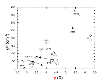 Figure 4.10. Relationship between electron binding energies (computed at the Koopmans' theorem level) and the dipole moment for several dipole-bound anions.
 - The FFD model overestimates binding energies, but, when Coulomb and exchange potentials of inner shell electrons are included, the model is reasonable but not highly accurate.
- Dispersion interaction of the excess electron with the remaining electrons is usually important to include if one wants accurate results and especially for very weakly bound anions.
- Relaxation of the neutral's orbitals caused by attaching an excess electron is usually small. As a result, a Koopmans' theorem treatment of the excess electron using specially designed basis sets [[179]] followed by inclusion of the dispersion interactions [[98], [180]] between the excess electron and the others is often adequate.
- When electron binding energies exceed the spacings between rotational levels of the
molecule, it is safe [[181]] to neglect non-Born-Oppenheimer (non-BO) couplings that can induce electron ejection.
Likewise, when the binding energy exceeds vibrational level spacings, it is usually
safe to neglect vibrational non-BO couplings that can lead to electron loss.
An example from Professors Carl Lineberger and Torkild Andersen of a case in which rotation-electronic coupling causes electron ejected is illustrated in Fig. 4.11 where the rates of electron loss [[182]] from the dipole-bound excited state of NC-CH2- are plotted as a function of the rotational quantum number that corresponds to tumbling of the C-CN axis. The various sets of data shown correspond to different values of the K quantum number relating to spinning of the H2C- group.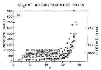 Figure 4.11. Plots of the rates of electron detachment from H2C-CN- induced by non-Born-Opppenheimer coupling to the rotational motion.
 - Even species that form valence-bound anions may also form dipole-bound states if their dipole moments are large enough.
- It is very rare to observe bound excited states for dipole-bound species; only for species with very large dipole moments (e.g., > 10 Debyes) is the binding for excited states as large as a few cm-1.
- The range of molecules that have been determined to form dipole-bound states is large and growing. In addition to those mentioned above, such states are formed in clusters such as (H2O)n-and (HF)n- [[122], [123], [171], [183]], in nucleic acid bases such as uracil [107] and thymine [108], and in many zwitterionic species.
Before closing this Section, I want to mention another theoretical contribution to understanding the dynamical stability of dipole-bound anions. The Lineberger and Brauman groups teamed up [[184]] to study the spectroscopy of the acetaldehyde enolate anion H2CCHO- that has a valence-bound ground state and a dipole-bound excited state. They resolved transitions that produce the dipole-bound state in various rotational levels labeled by the quantum numbers J and K. Because H2CCHO- is only an approximate symmetric top molecule, the use of these quantum numbers is not rigorously applicable. Nevertheless, the quantum number K measures (approximately) the angular momentum (and energy) for spinning about the a-axis shown in Fig. 4.12.
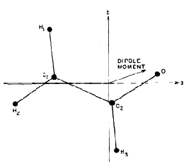
Figure 4.12. Principal axes (a, b, c) of H2CCHO.
The quantum number J labels the total rotational angular momentum.
For each of the rotational transitions involved in the valence-to-dipole electronic transition, these workers also determined the linewidth of the peak from which they inferred the rate of rotation-induced electron detachment. Professor David Clary developed a dynamical theory for estimating the rate of energy flow from the rotational motion of a molecular dipole into the electronic energy of the dipole-bound electron. Clary was able to use his theory to model [[185]] the linewidths that the workers of ref. 184 had assumed arose from autodetachment. His predicted linewidths (G) are shown if Fig. 4.13 and compared to those obtained experimentally in ref. 184.
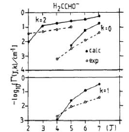
Figure 4.13. Linewidths of rotational levels (labeled by K and J quantum numbers) of dipole-bound state of H2CCHO-.
Clary was also able to apply his theory to the linewidths observed in ref. 182 for rotational lines in the dipole-bound state of H2CCN-. His results are compared to the experimental linewidths in Fig. 4.14.
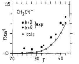
Figure 4.14. Linewidths of rotational levels (labeled by J and K quantum numbers) for dipole-bound state of H2C-CN-.
The theoretical model of Clary seems to be very capable of reproducing the linewidths observed for the various rotational levels of both H2CCN- and H2CCHO-. This lends credibility to the interpretation that the linewidths arise from Heisenberg broadening due to the rotation-induced detachment process. Moreover, the fact that the linewidths seem to be rather independent of the K quantum number but strongly dependent on the J quantum number tells us that it is not spinning of the H2C- group but tumbling of the molecular dipole that causes the detachment.
II. Binding an Electron to Quadrupolar Molecules
Here, we will primarily deal with the theoretical differences between dipole and quadrupole binding and mention a few attempts to identify species that might be classified as quadrupole-bound.
A. Is There a Critical Value for the Quadrupole Moment?
The interaction of an electron with a point quadrupole moment of magnitude Q is governed by the potential
V(r,q, f) = - Qe (3 cos2(q) -1)/(3r3).
The Schrödinger equation governing the motion of an electron in this potential is
[-h2/2mer-2 ∂/∂r (r2 ∂/∂r) + L2 /2mer2 ] y(r,q, f)- Qe (3 cos2(q) -1)/(3r3) Y = E Y.
The angular part of the quadrupole potential, which is proportional to the L = 2 spherical harmonic, is a quantity that ranges from -1/3 to +2/3. So, at all points in r, q, f space, the potential - Qe (3 cos2(q) -1)/(3r3) is less negative than the isotropic potential
V0 (r) = -Qe/r3.
Therefore, for any wave function Y (r,q, f), the expectation value of the spherical Hamiltonian
H0 = T + V0
will lie below the expectation value of the quadrupole Hamiltonian H = T + V:
<H0> < <H>.
The main question is whether bound states of H exist and, if so, for what values of Q.
Landau and Lifschitz [[186]] demonstrated that, because of the attractive 1/r3 form of the potential, and independent of the magnitude of Q, H0 has bound states of infinitely negative energy in which the electron is bound infinitesimally close to the origin. They speak of the electron falling into the origin of the potential. So, unlike the dipole case for which m has to exceed 1.625 D for bound states to exist, the point quadrupole potential can support bound states for any Q > 0.
However, neither the potential V nor V0 shown above is a realistic representation of the electron-molecule interaction as r approaches zero; any real molecule has inner-shell electrons whose repulsions will act to offset the attractive V (or V0) at small r. Hence, it is of more relevance to consider whether H or H0 can support bound states but with V or V0 cut off at small-r by a repulsive potential chosen to represent the core and other valence electrons. Here we will consider the simplest realistic cut off, an infinite wall at r = rc. Specifically, we consider case of H0 with the quadrupole V0 applying for r > rc and with V0 = ∞ for r < rc. Moreover, we will treat only L = 0 because this case is expected to produce the lowest-energy states. Introducing Y = F/r into the Schrödinger equation gives the following equation for F:
-h2/2me ∂2F/∂r2 -Qe/r3 F = E F.
The function F is normalized so that
![]()
and F vanishes at r = rc because of the infinite wall. Let us now try to determine whether this equation can have bound states.
Because the Hamiltonian H0 is bounded from below (since we cut V0 off at rc), we know that the lowest exact eigenvalue of H0 will
- lie below the expectation value of the above Hamiltonian H0taken for any trial functionFtrial and
- lie above the minimum in the potential –Qe/rc3.
We now choose the following trial function [[187]]
Ftrial = C(r-rc)2 (r-3rc)2 for rc <r < 3rc
and Ftrial = 0 elsewhere, where C is the normalization constant. It can be shown that the expectation value of H0 for this Ftrial is equal to:
<Ftrial |H0|Ftrial> = {h2/2me (656/105) 1/rc2 -Qe I/rc3}(315/256),
where I is the following positive integral:
![]()
The factor h2/2me (656/105) 1/rc2(315/256) is the kinetic energy and -Qe I/rc3(315/256) is the potential energy. Because the positive kinetic energy contribution to <Ftrial |H0|Ftrial> scales as rc-2 and the negative potential energy contribution scales as rc-3, it is clear that the total energy can be negative if Q is large enough or rc is small enough.
This analysis shows that a quadrupole potential of any strength (Q) can bind an electron if the repulsion due to inner shell electrons is weak enough (i.e., if rc is small enough). Conversely, a molecule of any size (i.e., having any number of inner-shell electrons as characterized by rc) can bind if its quadrupole moment is sufficiently large. Thus, unlike the dipole case, there is no critical value for the quadrupole moment.
The fundamental differences among the cation or neutral (having long-range Coulomb attraction scaling as r-1), the dipole (having long-range attraction scaling as – r-2), and the quadrupole (having long range attraction varying as - r-3) cases are important to note. The reason these three cases are so different in the kind of bound electronic states they support is that the radial kinetic energy operator (-h2/2mer-2 ∂/∂r (r2 ∂/∂r) + L2 /2mer2 ) scales as r-2. It is the combination of the - r-1 scaling of the potential and r-2 scaling of the kinetic energy that produces the infinite series of bound states appropriate to the Coulomb potential (e.g, in the hydrogenic atoms and in Rydberg states of molecules). Likewise, it is the – r-2 scaling of the potential and the r-2 scaling of the kinetic energy that produces the critical condition on the dipole moment below which no bound states exist. Finally, it is the –r-3 potential scaling and the r-2 kinetic energy scaling that produces bound states for any and all magnitudes of the quadrupole potential (as long as there is no short-range repulsion).
B. Real Molecules that Quadrupole Bind
As in the case of anions that one says are dipole-bound, it is difficult if not impossible to find a species for which one can confidently say the excess electron is purely quadrupole bound. For example, the (BeO)2- anion considered by Professors Jordan and Liebman [[188]] and more recently by Gutowski and Skurski [[189]] has been suggested to be a quadrupole bound anion. At its equilibrium geometry, the neutral (BeO)2 is a rhombus and has zero dipole moment but has a quadrupole tensor with principal eigenvalues of 36.4, 0.4, and –36.8 DÅ. In the ground state of the (BeO)2- anion, the excess electron is bound by more than 1 eV in an orbital that is shown in Fig. 4.15.

Figure 4.15. Orbital holding the excess electron in (BeO)2- [189].
If one were able to show that a quadrupole potential consistent with the above principal values, cut off by Coulomb and exchange interactions of the inner shell orbitals appropiate to (BeO)2), would reproduce the above orbital and the 1 eV binding energy, one would have a strong case for claiming a dominance of quadrupole binding. However, it is likely that a significant part of the 1 eV binding is due to valence-range attractions in the regions of the two Be+2 centers. So, although, in my opinion, it is valid to categorize (BeO)2- as quadrupole bound because the longest range potential experienced by an excess electron is indeed the charge-quadrupole potential and the d-symmetry charge distribution of the excess electron (see Fig. 4.15) is consistent with this L = 2 potential, there are other potentials that contribute to the total binding energy. That it, just as was the case for dipole-bound anions, potentials other than the longest-range attractive potential can contribute substantially to the total binding energy.
Also as in the case of dipole binding, one has to be careful not to call a species quadrupole-bound simply because it has no net dipole moment. To illustrate, consider a hypothetical molecule consisting of the following salt: Na+ -O-(CH2)n-O- Na+. When this species achieves a highly extended (i.e., quasi-linear) and symmetrical structure it likely has zero (or a very small) dipole moment because the two oppositely directed dipoles cancel one another. If one adds one excess electron to this molecule to form Na+ -O-(CH2)n-O- Na, does one have a quadrupole-bound anion or a dipole-bound anion? I prefer to call this a dipole-bound species for two primary reasons:
- As the number of methylene units grows, one finds the electron binding energy in Na+ -O-(CH2)n-O-Nato reach an asymptotic value near that of H3C-O- Na in which the excess electron is dipole-bound (albeit with significant contribution from valence-range attraction in the region of the Na+ ion). If Na+ -O-(CH2)n-O- Na were quadrupole-bound one would expect the binding energy to grow considerably as the number of –CH2- units grows because the quadrupole moment would increase.
- The radial exetent of the orbital one finds in Na+ -O-(CH2)n-O- Na does not extend over the entire framework of this molecule and thus does not extend over the entire set of charges that comprise the quadrupole.
For these reasons, I prefer to view Na+ -O-(CH2)n-O- Naas a dipole-bound anion that is perturbed by another distant dipole.
In carrying out successful theoretical calculations on quadrupole-bound anions, it has been found to be necessary to follow essentially the same steps as when treating dipole-bound anions. In particular, it is necessary to use the extra diffuse basis sets [50] described in Chapter 2 Sec. I and to include electron correlation (at least the dispersion interaction of the excess electron with the other electrons) effects. These steps are needed because the orbital occupied by the excess electron in the quadrupole-bound cases is large and diffuse and not necessarily localized on an atomic center as in the dipole-bound cases.
Other molecules that have been suggested to form quadrupole-bound anions include: CS2 [[190]], the anti-conformer of succinonitrile (NC-CH2-CH2-CN) [[132], [191]], p-di-nitro-benzene [[192]], and the rhombic isomer of (NaCl)2 [[193]]. The orbital into which the excess electron binds in the succinonitrile case [[194]], which arose from a collaboration among the Bowen, Compton, and Schermann-Desfrançois groups, is shown in Fig. 4.16 where we also show how the electron binds when this molecule adopts its less symmetric conformer and thus possesses a large dipole moment.
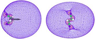
Figure 4.16. Dipole-bound orbital of the polar conformer of succinonitrile (left) and quadrupole-bound orbital of the same molecule in its anti conformation (right).
However, as with (BeO)2‑, it may be difficult to show in a convincing manner that the charge-quadrupole attraction is the dominant contributor to determining the binding energy even for some of the species just mentioned. For these reasons, we prefer to use the terms dipole-bound and quadrupole-bound to label the longest range potential that contributes to electron binding but to realize that other shorter-range potentials also often play significant roles in determining the total electron binding energy as well as the orbital containing the excess electron.
III. Binding Through Higher Moments
One can, of course, imagine constructing molecules such as clusters of alkali halide molecules that, because of the high symmetry or the cluster, possess both zero dipole and zero quadrupole moments. For such clusters, it may be that an excess electron can still be bound. However, again, and much in line with what I said above about dipole and quadrupole binding, one must be careful to conclude that the binding arises from higher-order moment of the charge distribution of the neutral cluster rather than via a more local binding to one of the fragments within the cluster. In this Section of this Chapter, we will not go beyong dipole and quadrupole binding when considering permanent moments of the charge distribution. Instead, let us turn our attention to binding that can occur due to the excess electron inducing moments in the parent molecule's charge distribution.
The Schermann-Desfrançois research group has examined [[151]-[163]] many species that bind electrons through dipole- and quadrupole- potentials, and, as I mentioned earlier, they have developed a flexible and powerful model [[195]] in terms of which to understand and predict such binding. In their model, the long-range attractive potential is taken to be a sum of dipole Vm, quadrupole VQ, induced-dipole Va, and other multipole potentials. An example of this potential appropriate to a symmetric-top molecule interacting with an electron is shown below
Vm(r,q) = -mcos(q)/r2 [1-exp(-(2r/m)3)]
VQ = -Q(3cos2(q)-1)/(4r3) [1-exp(-(2r/Q1/2)5)]
Va(r,q) = apar cos2(q)/(2rpar4) [(rpar/r)8 - (rpar/r)4]
+ aper(1- cos2(q))/(2rper4) [(rper/r)8 - (rper/r)4].
Here, apar and aper are, respectively, the components of the polarizability parallel to and perpendicular to the molecule's unique moment of inertia and q is the angle between that axis and the electron's position vector. The potential expressed in this form is in atomic (Hartree) units as are the radial position (Bohrs), dipole moment and polarizability parameters. We note that the dipole and quadrupole terms in the multipole potential are multiplied by short-range repulsive cut-off potentials that decay exponentially with r with parameters that depend on the values of the dipole and quadrupole moments, m and Q, respectively.
Through such model potentials, these workers have been able to examine, in a very efficient manner, a wide variety of anions and dianions that bind electrostatically. One of the keys to the success of such a model is the replacement of the usual ab initio (i.e., Coulomb and exchange) inner-shell short-range repulsion potential by the exponential cut-off functions that contain physically motivated parameters. However, this approach must also employ basis sets that are capable of locating the excess electron's density where the attractive potential directs it; in other words, diffuse and extra diffuse basis functions are usually also needed when this kind of calculation is carried out. A contour plot of the dipole-bound orbital of NCH- resulting from such a calculation is shown in Fig. 4.17.
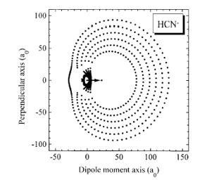
Figure 4.17. Contour plot for the dipole-bound orbital of NCH- with the positions along the x and y axes given in atomic (i.e., Bohr) units.
Of course, there has also been work done on binding electrons via charge-induced dipole (i.e., polarization) interactions that has not used the kind of model potential discussed above. For example, Professor Piotr Skurski et al [[196]] examined electron binding to 9-acridinamine (Fig. 4.18), which has a dipole moment of 3.1 D, so it should be able to bind an electron via charge-dipole interactions. However, they found that the binding energy of 6 cm-1 computed at the Koopmans' theorem (plus orbital relaxation) level, which includes the charge-dipole interaction, was cancelled by the second-order correlation contribution to the EA excluding the dispersion interaction between the attached electron and the other electrons. So, until the dispersion or van der Waals interaction energy is considered, this species was predicted to be unbound. The second-order dispersion interaction was found to be 20 cm-1 and thus ultimately responsible for the final positive EA of this molecule.
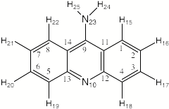
Figure 4.18. The 9-acridinamine molecule whose anion is claimed to be dispersion-bound.
For this reason, ref. 196 calls this a dispersion-bound anion (i.e., an anion resulting from the r-6 dispersion coupling of the excess electron and the remaining electrons of 9-acridinamine).
The anion and dianion of fullerene-type carbon clusters have also been treated by Professor Bob Compton's group [[197]] in terms of a dominant polarizability-based potential, and the author's group has used such a model [[198]] to study the effect of electron correlation in C602-. For example, in the Compton group's study of C84-, the one excess electron is modeled in terms of an attractive potential of the form -a/2r4, where a is the polarizability of C84 (ca. 120 Å3) and r is the distance from the electron to the center of the C84 molecule. In contrast, for the dianion C842-, the second excess electron is described in terms of a potential -a/2r4 + e2/r, the latter factor representing the Coulomb repulsion of the second excess electron due to the C84- anion. This potential, which displays a characteristic Coulomb barrier near r = 8 Å, is shown in Fig. 4.19.
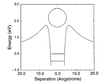
Figure 4.19. Model attractive -a/2r4 and Coulomb repulsive e2/r potential appropriate to an electron interacting with C84-. The size of the C84 framework is depicted by the spherical object in the center.
Solving the Schrödinger equations for the motion of the first excess electron in the presence of the -a/2r4 potential produces the bound state lying 3.14 eV below the energy of the neutral C84. The bound state found for the second excess electron lies 0.44 eV below the energy of the mono-anion, when the -a/2r4 + e2/r potential is used [197]. When this same kind of model is applied to C60, one finds the C60- anion to lie 2.65 eV below C60, but the C602- dianion is predicted [198] to be slightly unstable with respect to C60-.
Thus far in this Chapter we have overviewed the so-called point dipole and fixed finite dipole models that describe the interaction of an excess electron with a dipolar molecule. We discussed various dipole-bound species and the special theoretical steps that need to be taken to study them. We also discussed examples of binding an electron (primarily) by the electron-quadrupole potential as well as binding that is likely due to the polarization (i.e., charge-induced-dipole) potential.
Although dipole- and quadrupole-bound anions may seem rather esoteric, they are likely to be more widely appreciated as the number of workers who have encountered them grows. Their very diffuse excess-electron charge distribution likely makes it difficult if not impossible to form these anions in condensed-phase environments (e.g., in liquids or solids). For example, in liquid water, the hydrogen-bonding network that exists and acts to confine water molecules to a narrow range of orientations makes it rare for several water molecules to be found in a quasi-linear orientation of very high dipole moment such as that shown in Fig. 4.20 for the water tetramer anion.
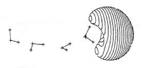
Figure 4.20 Minimum-energy structure of (H2O)4- also showing the orbital occupied by the excess electron.
Thus, is it not likely that such a dipole-bound water tetramer unit will spontaneously form and persist long enough to be studied in bulk water. However, this anion (and other (H2O)n- anions) can form in water vapor and on the surfaces of liquid or solid water where the positive ends of H2O dipoles can be exposed (i.e., not surrounded by other water molecules) and thus able to attach an electron. Moreover, we know that water tetramer anions can occur even in bulk water if the four H2O molecules are given enough time to allow thermal fluctuations to orient them with their dipoles directed tetrahedrally inward; we are speaking, of course, about the solvated electron in water. The attractive potential that binds the solvated electron is comprised (largely)of the dipole potentials of the four surrounding H2O molecules directed inward toward the center of the solvation site as well as polarization potential due to the remaining water molecules.
It is likely that highly polar clusters of polar molecules, when favored thermodynamically or allowed to form by thermal fluctuations, will be observed to form dipole (or quadrupole) bound anions. Especially at surfaces of liquids or solids, at steps or defects on surfaces, or in gas-phase nanoscopic clusters, such local groupings of constituent polar molecules will arise and, therefore, dipole-bound electrons will be observed.
IV. Double-Rydberg Anions
The next class of anions to be discussed derives from the electrostatic potential provided by a positively charged molecule to which two electrons are bound. Specifically, we consider a class of molecular anions that arises by placing two extra electrons into a Rydberg orbital of a closed-shell molecular cation. An example that we discussed earlier in the text is (NH4)-, which can be viewed as a closed-shell NH4+ cation with two electrons attached to its lowest-energy Rydberg orbital (Fig. 4.21).

Figure 4.21. Rydberg orbital of NH4 showing how the orbital extends beyond the valence range of the nitrogen and hydrogen atoms.
Molecules that contain closed-shell cationic sites such as protonated amines R-NH3+, protonated alcohols R-OH2+, and protonated thiols R-SH2+ can bind an electron to form a Rydberg neutral species [[199]]. In all of these Rydberg-orbital cases, the long-range Coulomb attraction of the cation site is a dominant contributor to binding, and the repulsions of the inner-shell electrons provide the balancing forces to the Coulomb attraction. The resultalt potential generally supports a series of electronically bound Rydberg states and, as we discussed in Chapter 2, their electron binding energies fit the formula E = -13.6 eV(Zeff2/(n-d)2). In Fig. 4.22 we show two such Rydberg orbitals (ground and excited) in which the orbitals are bound to the protonated amine site in
+ H3N-(CH2)3-SS-CH3.
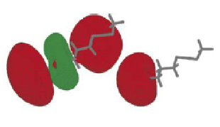
Figure 4.22. Ground (right) and excited (left) Rydberg orbitals of H3N-(CH2)3-SS-CH3.
As in the simpler NH4+ case shown in Fig. 4.21, one electron can be attached to either of these (or higher) Rydberg orbitals to form a neutral Rydberg molecule. On the other hand, if two electrons are placed into one (or two) of these Rydberg orbitals, a so-called double-Rydberg anion is formed. Professor Kit Bowen was the first to experimentally identify such anions [[200]] and Professors Vince Ortiz and Maciej Gutowski studied them theoretically [[201]], but at least one of them (NH4-) had been examined earlier by Professor Josef Kalcher [[202]].
The neutral Rydberg species tend to have very low barriers to fragmentation [[203]]. For example, the ground Rydberg state of R-NH3 decays to R-NH2 + H over a barrier of but a few kcal mol-1. The low barrier in such cases is expected because only a single electron's orbital occupancy must be altered to effect such a cleavage. In the example just cited, the electron in the Rydberg orbital must change to occupy the H atom 1s orbital. In contrast, the anionic double-Rydberg species have larger barriers to bond cleavage and are thus geometrically more stable. The stability [203] derives in part from the fact that two electrons' orbital occupancy must change to fragment the anion. For example, to break NH4- apart into NH3 + H-, two Rydberg electrons must change orbital occupancy to two H 1s electrons.
Two more things that are important to note about Rydberg orbitals and double-Rydberg anions are
- That the large radial extent of Rydberg orbitals causes them to overlap with (and thus couple to) orbitals (bonding, lone pair, and anti-bonding) that may be rather distant from the functional group holding the postive charge to which the Rydberg orbital is bound. This characteristic causes Rydberg orbitals to offer greater possibility for inter-orbital electron transfer than one might expect based on experience with conventional valence-size orbitals.
- That the strength of the mutual Coulomb repulsions between the two electrons occupying a Rydberg orbital is high.
To illustrate the importance of the latter point, we note that a neutral Rydberg species such as NH4 binds its excess electron by ca. 4 eV yet the corresponding double-Rydberg anion NH4- binds its second electron by only 0.4 eV. Thus, the Coulomb repulsion between the two Rydberg-bound electrons must be ca. 3.6 eV. So, any treatment of the electronic structure of NH4- must treat this (strong) interaction energy to better than 5% to be able to determine the electron binding energy within 50%.
This suggests that any successful treatment of double-Rydberg anions must allow for a correlated treatment of at least the two electrons in the Rydberg orbital. For example, in studying the nominally a12 (in tetrahedral symmetry) configuration of an anion such as NH4-, if one were to employ a single-configuration electronic wave function in which the two excess electrons occupy a1a and a1b spin-orbitals, the energy of NH4- turns out [[204]] to lie above that of neutral NH4. In other words, at the Hartree-Fock level of theory, double-Rydbeg anions are often predicted (incorrectly) to be unstable with respect to electron loss. The problem is that the HF description does not allow for the two Rydberg electrons to correlate their motions and thus lower their total energy. To account for some degree of electron correlaton, it is common to use wave functions that contain both a12 and t2 orbital occupancies for the two electrons that nominally occupy the Rydberg orbital. This allows one to combine the t-symmetry p-like Rydberg orbitals with the a1 s-like orbital to form polarized orbital pairs as discussed in Chapter 2. By using such a multi-determinant wave function, one allows the two excess electrons to undergo angular correlation as they occupy (a1 ± x t) polarized orbital pairs and thus avoid one another and lower the total energy. Again we emphasize that including such correlations is essential to obtaining a qualitatively correct description of the two Rydberg electrons in double-Rydberg anions; a wave function that contains only one configuration (e.g., the a12 configuration for NH4-) does not even predict the anion to be electronically stable.
In summary, whenever one has a closed-shell positively charged (+1, +2 or higher charged) functional group in a molecule, one should anticipate that neutral Rydberg states (a manifold of them having electron binding energies fit by E = -13.6 eV(Zeff2/(n-d)2)) can be formed. One should also expect that double-Rydberg anions, in which two electrons occupy Rydberg orbitals, can be formed. The neutral Rydberg species will bind their excess electron strongly (ca. 4 eV for Z = 1 ions) but will have low barriers to bond cleavage. The double-Rydberg species will bind their (second) excess electron less strongly (ca. 0.4 eV) but will have higher barriers to bond cleavage.
V. Zwitterion-Bound Anions
Cation-site binding also occurs in a class of anions formed when an excess electron is attached to a zwitterion tautomer of a molecule such as an amino acid (e.g., H3N+-CHR-COO-). Again, the electron occupies an orbital that is localized primarily on the cation site within the zwitterion neutral. For example, in arginine and urea, the cation-site-localized orbitals into which the excess electron is attached are as depicted in Fig. 4.23 from the laboratory of Professor Skurski [[205]].
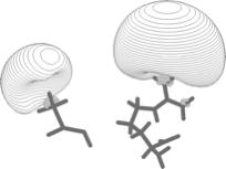
Figure 4.23. Cation-site orbitals holding the excess electron in anions formed from zwitterions tautomers of urea (left) and arginine (right).
When viewing members of this class of anions, one probably wonders why they are not classified as either dipole-bound (is the zwitterion not a giant dipole?) or Rydberg-bound. They should not be put into the dipole-bound class for two reasons that were disussed in Chapter 4. First, as the distance between the positive and negative sites of the zwitterions increase, the dipole moment grows, and so the electron binding energy should continue to grow in parallel. However, this is not what happens; instead, as the distance grows, the electron binding energy approaches that of the cation site. So, it might be argued that we should view zwitterions-bound anions as Rydberg-bound species that are perturbed by a nearby negative charge. However, because the zwitterions moiety is so prevalent in chemistry, I choose to keep these anions within their own category.
In zwitterion-derived anions, the binding energy of the excess electron is determined primarily by two factors:
- the intrinsic binding strength of the cation site, which is similar to the binding energy in the corresponding Rydberg neutral (e.g., 3-4 eV), and
- the Coulomb repulsion (e2/R = 14.4 eVÅ/R(Å)) exerted on the excess electron attached to the cation site by the negatively charged site of the zwitterion, which depends on the distance R between the positive and negative sites (e.g., this Coulomb repulsion is ca. 1.9 eV in arginine and 3.7 eV in urea).
This suggests that the longer the chain separating the two charged sites in the zwitterion, the stronger the net binding energy should be to the cation site and the more compact the orbital occupied by the excess electron. Indeed, such trends are observed in numerous situations where internal Coulomb repulsion plays a crucial role in determining the electron binding energy.
Some molecules, such as amino acids, have both zwitterionic and canonical (i.e., containing no zwitterion site) structures. In such cases, it may be possible to bind an excess electron in either of two ways: to the dipole potential of the canonical isomer, or to the cation-site of the zwitterion tautomer. An example from Professor Piotr Skurski's lab is shown in Fig. 4.24 where arginine's canonical (left labeled C) and zwitterion (right labled Z) neutral (N) and anionic (A) species are shown [[206]].
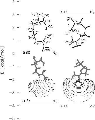
Figure 4.24. Canonical (left) and zwitterion (right) neutral (top) and anion (bottom) tautomers of arginine, with the orbital occupied by the attached electron shown and the relative energies indicated.
Notice that the orbital occupied by the excess electron in the zwitterion case looks very much like the orbital occupied by this electron in the canonical case, in which the electron is dipole-bound. So, both dipole-bound and zwitterions-bound orbitals can be diffuse and are localized on the positive end of the molecule, so it is often difficult to distinguish between the only two by looking at the orbitals.
Another example [[207]] of zwitterion binding of an electron is offered by the novel molecule shown in Fig. 4.25. It turns out that this species' lowest-energy tautomer is its zwitterion tautomer (Z); this is rather unusual because most molecules that possess zwitterion structures have non-zwitterion tautomers as their lowest-energy structures.
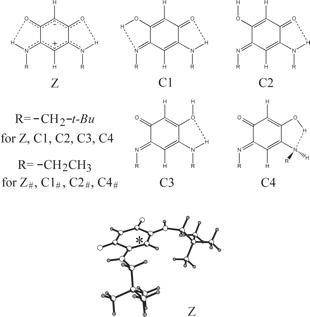
Figure 4.25. The novel zwitterion Z is the lowest energy neutral structure of this molecule.
Even when rather bulky –CH2-t-butyl groups are appended to the cationic side of the zwitterion, an electron is able to bind to this site in the orbital shown in the top of the Fig. 4.26.
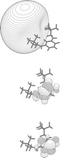
Figure 4.26. The zwitterion Z shown in Fig. 4.25 can bind an electron via dipole binding (top orbital). The middle orbital is a p* orbital that lies higher in energy than the zwitterion orbital, and the bottom orbital is the neutral's highest occupied p orbital.
Chapter 5. Multiply Charged Anions
In this Chapter, we will discuss doubly and triply charged molecular anions, some of which are
- electronically stable but geometrically metastable (e.g, MgF4-2and TeF8-2 have very large > 3 eV vertical electron binding energies but are thermodynamically unstable with respect to dissociation to form F- and MgF3- or TeF7-, respectively) , others that are
- electronically metastable (e.g., SO4-2, PO4-3 spontaneously lose an electron in the gas phase), and yet others that are
- electronically and geometrically stable (e.g., . -OOC-(CH2)n-COO- for large enough n).
Many, but not all, of these species use valence (as opposed to Rydberg or dipole) orbitals to bind their electrons. For the ions that are electronically metastable, the issue of their lifetime with respect to electron loss will also need to be addressed, and new theoretical tools designed to handle such non-stationary states must be discussed as I do toward the end of this Chapter.
To set the stage for discussing under what circumstances two or more excess electrons can bind to a molecule, we remind the reader that the ground electronic states of atoms bind a single excess electron by no more than ca. 3.5 eV. This, in turn, suggests that no valence site in a molecule will bind an excess electron by more than approximately this same amount, although delocalization and resonance effects can alter the situation somewhat. Because the Coulomb repulsions between two negative charges R Å from one another is given by 14.4 (eV Å)/R(Å), this means that two negative sites closer than 4.1 Å will be subject to electron autodetachment because their mutual Coulomb repulsion will exceed the expected maximum intrinsic electron binding strength of 3.5 eV. In fact, such Coulomb interactions are what cause atomic dianions (e.g., O2-) and very small molecular dianions such as O22- to not be electronically stable as isolated species. So, we expect to find multiply charged anions that are electronically bound only when the atoms from which the ion is constructed have high intrinsic electron binding strengths and when the ion's geometry keeps the negative sites far from one another.
In this Chapter, we discuss several classes of dianions and trianions that have been subjected to considerable study in recent years and we introduce some of the special theoretical methods that must be used to probe their electronic structures. Some especially useful soureces of material on multiply charged anions are the web sites of Professor Lenz Cederbaum, Professor Lai-Sheng Wang, and Professor Alex Boldyrev whose groups have carried out a very large number of experimental (Wang) and theoretical (Cederbuam and Boldyrev) studies of these species. Let us now examine the first category of such multiply charged anions.
I. Binding to Polar Molecules
A. What the PD and FFD Models Suggest
When the fixed finite dipole (FFD) model is reconsidered for binding two electrons, one faces the following Schrödinger equation [[208]]:
{- h2/2me (∇12 + ∇22) –q e2/|r1| +q e2/|r1-R|–q e2/|r2| +q e2/|r2-R| + e2/|r1 – r2| }Y = E Y,
where q is the charge on the two centers and R is their separation. Introducing scaled electron radial coordinates: r1 = r1/q and r2 = r2/q as well as the scaled internuclear distance R = r/q, transforms the above equation into:
q2{- h2/2me (∇12 + ∇22) –e2/|r1| + e2/|r1-r|– e2/|r2| + e2/|r2-r| +q-1 e2/|r1 – r2| }Y = E Y,
where the radial derivatives in the ∇2 operator now refer to rj-derivatives. The Hamiltonian H on the left side of the above equation can be written as:
H/q2 = h(1) + h(2) + q-1 e2/|r1 – r2|,
where h(1) and h(2) are the FFD Hamiltonians for the two separate electrons:
h(1) = -h2/2me ∇12– e2/|r1| + e2/|r1- r| ,
h(2) = -h2/2me ∇22– e2/|r2| + e2/|r2 – r2|.
In the limit, q → ∞, R → 0, with qR = r finite, H/q2 becomes h(1) + h(2), so the solutions to
(H/q2) Y = e Y
become, in this limit, antisymmetrized products (i.e., Slater determinants) of solutions of the one-electron FFD equation
h fj = ej fj,
multiplied by a or b spin functions. The lowest-energy such solution would be of the form:
Y = |f1a(r1) f1b(r2)|,
with the vertical lines denoting the Slater determinant. The total energy of this ground-state solution of the two-electron FFD model in the large-q limit is given as the sum of the two energies of the one-electron FFD problem:
E/q2 = 2 e1.
This shows that as the FFD model approaches the PD limit of large q and small R with fixed qR (i.e., fixed dipole moment m), the conditions needed for two electrons to barely bind to form the lowest-energy state are that e1 be slightly negative. This is exactly the same condition needed for the one-electron PD model to critically bind. Hence, the critical dipole for binding two electrons to the PD is exactly the same as for binding one electron.
In contrast to these findings for the PD model, numerical calculations [[208],[209]] suggest that for the FFD model there is no unique critical m = q R value to achieve binding the second electron. Instead, for each q value, there is a critical m value, and there exists a rather strong dependence of mcritical on q as shown in Fig. 5.1.
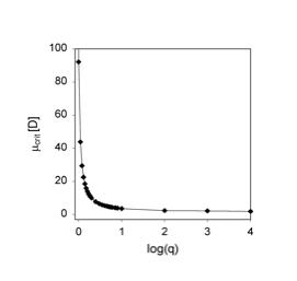
Figure 5.1. Plot of critical dipole moments for various q values within the FFD model [208].
Although it is not possible to glean from Fig. 5.1, the large-q limit for mcritical is indeed 1.625 D, as noted earlier. It turns out that there is another asymptote that arises in the FFD model; the minimum value of q for which a bound dianion exists. In this limit, one has mcritical→∞ as q → 0.91. This means that the center with charge +0.91 can bind two electrons but only if the other center of charge –0.91 is infinitely far away (and, thus m = qR is infinite). For comparison, when q = 1.0, two electrons can be bound to the +q center (to form H-) if the – q center is 19.19 Å distant (for which m = 92.17 D).
It may occur to the reader whether it makes sense to refer to a species as dipole-bound when it consists of two charges of magnitude q and opposite signs separated by such a large distance. Indeed it probably does not make sense to do so in this case. It is probably more reasonable to view the electrons bound to the +q charge as being polarized by the –q charge residing at R = 19.19 Å. In general it is difficult to give firm rules for when to call such species dipole-bound and when to call them anions that are polarized by a distant charge. However, as I pointed out in Chapter 4, a reasonably good rule of thumb is to refer to the system as dipole-bound if the radial extent of the wave function describing the two bound electrons exceeds the distance between the +q and –q charges. If the wave function lies primarily inside of this distance, it is more appropriate to refer to the system as an anion that is polarized by the –q charge. I refer the reader to our earlier discussion of systems such as –OOC-(CH2)n-NH3+ with an electron bound to the –NH3+ end. Such species are not dipole-bound but are Rydberg-bound with perturbation from the distant –OOC- group.
These examples introduce a concept that is important to appreciate when considering the stability of dianions- the role of Coulomb repulsion. It turns out that the critical distance Rc (and hence the critical dipole) for q values in the range 0.91 < q < 2 can be very well predicted by:
- first computing the electron binding energy for the second electron attached to the +q center (this we call the intrinsic binding energy of the +q center), and then
- reducing this binding energy by the Coulomb repulsion energy e2/R produced by the other center, where R is the distance to the –q center, and finally
- determining for what value of R the intrinsic binding energy will be totally offset by the Coulomb repulsion (this value of R is denoted Rc). As we will see later, competition between intrinsic binding and Coulomb repulsion plays a major role in determining the net stability of multiply charged anions. For example, one can predict the electron binding energies in dianions such as–OOC-(CH2)n-COO-by taking the intrinsic binding energy of a reference mono-anion such as –OOC-CH3 (ca. 3.2 eV) and subtracting the Coulomb repulsion between the two negatively charged centers. One can use this Coulomb model to estimate the (negative) electron binding of, for example, SO42- by taking the intrinsic binding energy of the HSO4- mono-anion and subtracting the Coulomb repulsion between two neighboring oxygen centers (i.e., 14.4 eVÅ/R(Å), where R is the O-O distance in SO42-).
B. Real Cases
To our knowledge, there have been no experimental observations of species that can be classified as dipole-bound dianions. Moreover, there has been only one theoretical prediction from Professor Skurski [[210]] of such a dianion, and the structure of this unusual species is shown in Fig. 5.2.
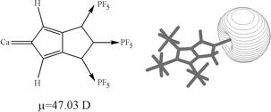
Figure 5.2. Structure of predicted dipole-bound dianion (left) and of the orbital (right) containing the two excess electrons. This orbital is localized on the Ca end of the molecule [210].
In this dianion, the second electron is bound by ca. 0.8 eV and resides in the same orbital as does the first excess electron. The relatively large binding energy once again suggests that shorter-range attractive potentials also contribute to the binding energy. This, of course, is not surprising considering that the underlying molecule shown above contains nominally a Ca+2 center.
II. Binding to Two Distant Sites in a Single Molecule
As discussed above, when considering the possibility of binding two electrons to two distinct sites in a molecule (e.g., two orbitals localized far from one another), one must consider the mutual Coulomb repulsion energy between the two anion sites. An excellent illustration of this effect is presented in the photoelectron spectra of dicarboxylate dianions [[211]] taken in the laboratory of Professor Lai-Sheng Wang. In these spectra whose results are summarizied in Fig. 5.3, mass-selected dianions are exposed to radiation having more than enough energy hn to detach one electron.
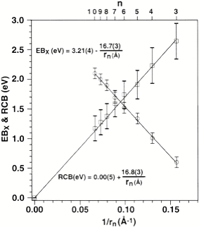
Figure 5.3. Measured detachment energies of dicarboxylates having various (n) CH2 units [211].
The kinetic energy KE of the detached electrons is then subtracted from the photon energy to obtain the electron binding energy EB = hn - KE as is conventional in photoelectron spectroscopy. These binding energies are determined for dicarboxylate dianions –O2C-(CH2)n-CO2- having various number of –CH2- units. In Fig. 5.3, the detachment energies of dianions –O2C-(CH2)n-CO2- of varying length (the Coulomb repulsion is thought to cause the chain to adopt an all-trans elongated geometry in the gas-phase) are plotted as a function of the inverse of the distance rn between the two carboxylate centers. The linear slope is interpreted in terms of the intrinsic binding energy of a R-CO2- anion (the y-axis intercept of ca. 3.2 eV) being lowered by the Coulomb repulsion e2/rn between the two anionic sites to produce a net electron binding energy.
This Coulomb model has proven to be very useful both in interpreting experimental data on such non-proximate dianions [211] and in theoretically predicting binding energies of dianions [[212]]. For example, the author's group extended earlier studies of dipole binding to LiCN and (LiCN)n clusters to a model system [[213]] consisting of two (LiCN)2 units oriented oppositely and separated by an H-C≡C-H spacer: (LiCN)2 H-C≡C-H (NCLi)2. They knew that each (LiCN)2 unit would bind an excess electron by 1.35 eV (at the Koopmans' theorem level), and they found that
- the (LiCN)2H-C≡C-H (NCLi)2-1anion has two nearly degenerate (gerade and ungerade) states that bind the electron by 1.3 eV, which is not surprising based on the above binding energy for (LiCN)2- ;
- the (LiCN)2H-C≡C-H (NCLi)2-2binds its second electron by 0.8 eV.
The 0.5 eV difference between the anion and dianion electron binding energy is consistent with a Coulomb repulsion of two negative charges 29 Å from one another. The distance between the two Li centers in the (LiCN)2 H-C≡C-H (NCLi)2-2 dianion is 26.2 Å. Clearly, the fact that the orbital centroids of negative charge are displaced somewhat from the Li canters suggests that the Coulomb repulsion is the cause of the 0.5 eV reduction in binding energy when comparing the anion and dianion.
Notice that in computing the Coulomb repulsion in the above dianions, we do not assume the molecular framework that separates the two anion centers offers any dielectric screening. In fact, workers have routinely found that a simple Coulomb repulsion formula (e2/R) accounts for the decrease in electron binding energy, rather than a screened version e2/(eR). This may, at first, be surprising, given the fact that there are, for example in the above dicarboxylate cases, chemical spacer units separating the two carboxylate centers. However, unlike true dielectric screening situations such as one observes in solutions and in solids, there is not a three dimensional distribution of such –CH2- spacer units surrounding the two carboxylate centers. That is, dielectric screening results when two charges are separated and surrounded by polarizable molecules, not when they are only separated by a linear chain of polarizable groups for which the screening is minimal. It is for such reasons that the non-screened Coulomb formula is appropriate.
Before closing this Section, it is useful to again emphasize the distinction between dipole and quadrupole binding, and the (LiCN)2 H-C≡C-H (NCLi)2 model system offers a good example. In this molecule, we have two oppositely directed highly polar (LiCN)2 units. The entire (LiCN)2 H-C≡C-H (NCLi)2 molecule has no dipole moment, so it is tempting to consider its anion a quadrupole-bound anion because the quadrupole moment is the lowest non-vanishing moment of its charge distribution. However, when the orbital into which an excess electron is examined for this case (Fig. 5.4), one sees that each lobe of this orbital (acutally, both the sg and su orbitals show this behavior) has a radial extent that is small compared to the entire length of the molecule.
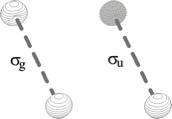 Figure 5.4. The sg and su orbitals of (LiCN)2 H-C≡C-H (NCLi)2 [213].
Moreover, one finds two nearly degenerate (i.e., within 4 cm-1 [213]) orbitals of sg and su symmetry, respectively. This means that the left- and right-localized orbitals L = 2-1/2 (sg + su) and R = 2-1/2 (sg - su) are nearly exact and degenerate eigenstates. Hence, this system really consists of two very weakly interacting dipole-bound systems rather than a quadrupole-bound system.
The lesson this example teaches is that it is important to ask whether an anion claimed to be bound by a moment of order n can more properly be viewed as being locally bound by moments of order n' < n that happen to cancel in the full molecule. As explained, the answer for (LiCN)2 H-C≡C-H (NCLi)2 is that the excess electron (s) are dipole-bound and that there are two (g and u) dipole-bound states. However, in the (BeO)2- anion discussed earlier, the authors found a stable anion of 2Ag symmetry (see Fig. 4.15), but their attempts [189] to identify a corresponding state of 2B2u symmetry showed that this state was not electronically stable. That is, the pair of g and u states is split by a very large amount that renders the higher-energy state not electronically stable. Hence, for (BeO)2-, the facts that one does not obtain a nearly degenerate pair of anion states and that the excess electron's orbital extends throughout the entire molecule (rather than being localized primarily on one or another end) support calling this a quadrupole-bound anion rather than a dipole-bound anion.
It is useful to again emphasize that it is important to be careful about calling anions dipole bound for similar reasons. For example, recall the FFD model discussed earlier when we talked about binding an electron to a dipole potential. We concluded that an electron could bind for a given value of the charge +q if the dipole moment m = qR exceeded 1.625 D. However, if for a given q-value the separation R between the two charges is much larger than the radial extent of the orbital to which the electron is bound, it is more appropriate to think of the system being an electron bound to a +q center that is polarized and destabilized by a –q charge at distance R. This observation suggests that although it may be proper to call ClNa- a dipole bound anion at the equilibrium distance Re, at much larger R-values, it is more appropriate to view it is an Na atom polarized by a Cl- anion at such larger distances.
III. Binding to Proximate Sites
Based on the discussion of Coulomb repulsion presented in earlier Sections, one might wonder if it is possible to form dianions (or other multiply-charged anions) in molecules where the two excess electrons reside in more proximate orbitals. The concern, of course, is that Coulomb repulsion would be so large as to cause either spontaneous ejection of one electron or fragmentation of the molecule's bonding framework. Such systems that have two or more excess electrons bound very near to one another include many ubiquitous species (e.g., SO4-2 and CO3-2 [[212], [214]]) as well as more exotic systems [[215], [216]] (e.g., TeF8-2 [[217]] and MgF4-2 [[218], [219]]). Of course, if the anion sites are too close, as they are in O2- or O2-2, the Coulomb repulsion is indeed too large to be offset by the intrinsic binding of each site. For this reason, O2- and O22- are not electronically stable; they decay by undergoing electron ejection. However, for the other systems listed above and many others, the intrinsic bindings and Coulomb repulsions are close enough to balancing to make such species fascinating to study. Let us consider a few examples.
For tetrahedral MgF4-2 studied in Professor Lenz Cederbaum's group [[220]] and square antiprism D4d TeF8-2 studied in Professor Alex Boldyrev's group [[221]], the intrinsic electron binding of each of the fluorine ligands as well as the delocalization of the two excess electrons over four or eight equivalent sites, respectively, more than offsets the Coulomb repulsion e2/RLL (RLL denotes the ligand-ligand distance) between the two excess charges nominally localized on the ligands. As a result, these dianions are (vertically) electronically stable by ca. 3 eV and 5 eV, respectively. That is, they bind their second excess electrons by amounts comparable to or in excess of the binding energies of halogens, which is quite remarkable.
However, these anions are not thermodynamically stable. In particular, they are not stable with respect to fragmentation into two singly charged anions. To illustrate, a plot of the energy of MgF42- as a function of one of the Mg-F distances, with all other geometrical parameters relaxed to minimize the energy, is shown below in Fig. 5.5.
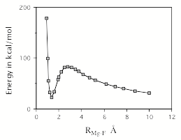
Figure 5.5. Energy of the ground state of MgF42- as a function of one Mg-F distance. Zero on the energy scale corresponds to F- + MgF3-.
Analogous plots for BeF42-, MgF42-, and CaF42- from Professor Lenz Cederbaum's group in which the energies of the corresponding mono-anions are also included [220] are shown in Fig. 5.6.
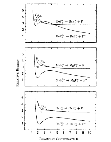
Figure 5.6. Energies of BeF42-, MgF42-, and CaF42- as one M-F bond length is stretched with all other degrees of freedom relaxed to minimize the energy.
It should be noticed that in the BeF42- case, the dianion becomes electronically unstable (i.e., has an electronic energy higher than that of the mono-anion) at moderately stretched Be-F bond lengths, so this dianion would undergo electron detachment before it dissociated into BeF3- + F-.
Of course, the lifetimes for fragmentation of such metastable dianions can be quite long both because the barriers to fragmentation (e.g., ca. 50 kcal mol-1 in the MgF42- example) can be high and because the fluorine ligands are too heavy to significantly tunnel through the barrier. We should note that the form of the potential curves shown in Figs. 5.5 and 5.6 are indeed of the e2/R form at large-R, illustrating the Coulomb repulsion between the F- and MFn-1- anions.
In contrast to the above electronically stable dianions, for SO4-2 and CO3-2 the internal Coulomb repulsion more than offsets the intrinsic binding strengths of the oxygen ligands, so these dianions turn out to be unstable with respect to electron loss. However, there is more to this interesting competition between Coulomb repulsion and intrinsic valence-range attraction that needs to be discussed because it illustrates another lesson about the roles of Coulomb repulsions in such anions.
If one imagines constructing any of the dianions mentioned above by bringing a second excess electron toward the corresponding mono-anion, one is lead to consider what potential this second electron would experience. Certainly, at long range, it would experience Coulomb repulsion caused by the mono-anion's negative charge. This repulsion would depend on the distance r of the second excess electron from the site (s) where the mono-anion's excess charge is localized. Such long-range repulsive potentials are shown on the right-hand sides of the figure displayed in Fig. 5.7 and were briefly introduced in Fig. 1.1 much earlier.
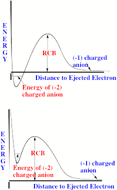
Figure 5.7. Effective potentials experienced by second excess electron when a stable (top) or metastable (bottom) dianion is formed.
As the second excess electron approaches closer, it eventually enters the region of space where the attractive valence-range potentials (e.g., near the fluorine or oxygen ligand orbitals in, for example, MgF42- or SO42-) are strong. In such regions, the total potential will be a sum of these short-range attractions and the Coulomb repulsions. If the former are strong enough, a deep attractive well will develop as shown in the top of Fig. 5.7, and the dianion will be stable with respect to the mono-anion plus a free electron. For example, such is the case for TeF8-2 and MgF4-2.
On the other hand, as is the case for SO4-2 and CO3-2, if the valence-range attractions are not strong enough, the total potential can display a minimum (as in the lower part of Fig. 5.7) that lies above the mono-anion plus free-electron asymptote. In such cases, the dianion will not be electronically stable, but can be metastable with a substantial lifetime. The lifetimes in such cases are determined by
- the height and thickness of the barrier shown in Fig. 5.7 (the barriers, in turn, are determined by the height of the repulsive Coulomb barrier (RCB)), and
- the energy at which the dianion state exists (determined by the intrinsic binding energy minus the Coulomb destabilization). We therefore see that the RCB both destabilizes the electron binding relative to the intrinsic binding energy and produces a barrier that may turn out to stabilize (i.e., with respect to autodetachment) the second excess electron if a metastable state results.
The lifetimes of such metastable anions have been estimated [212] by using a simple tunneling model in which the potential parameters shown in Fig.5.8 are:
- the height of the Coulomb barrier,approximated as e2/RLL, where RLL is taken to be the ligand-ligand distance;
- the energy of the dianion relative to that of the mono-anion plus a free electron, approximated as the ligand site's intrinsic binding energy reduced by the ligand-ligand Coulomb repulsion e2/RLL.
- A straightforward quantum integral is used to compute the probability of escape via tunneling through the Coulomb barrier.
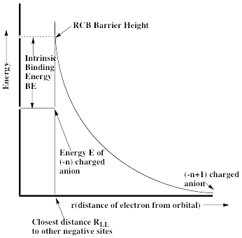
Figure 5.8. Simple Coulomb barrier model potential in terms of RLL, the ligand-ligand distance and the intrinsic binding energy [212].
When this kind of model is applied to SO4-2 and CO3-2, the dianions are predicted to be unstable by 0.75 and 1.50 eV and to have lifetimes of 2.7 x10⁻⁸ s-1 and 1.3 x10⁻¹¹ s-1, respectively. It turns out that these simple estimates are in reasonable agreement with estimates obtained by carrying out much more sophisticated ab initio quantum treatments on these same dianions. In the following Section, we discuss one of these more sophisticated methods.
Let's consider more examples of multiply-charged anions that are not electronically stable. One of the more interesting examples comes from Professor Lai-Sheng Wang's laboratory [[222]] where they studied the photoelectron spectum of the copper phthalocyanine (Pc) complex shown in Fig. 5.9.
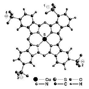
Figure 5.9. Copper phthalocyanine quadruply-charged anion studied if ref. 222.
The copper-centered highest occupied molecular orbital of this anion has its electron binding energy destabilized by its repulsive Coulomb interactions with the four surrounding negatively charged sulfonate groups. As a result, the energy of this 4-charged anion exceeds that of the 3-charged anion plus a free electron and thus this 4-charged anion corresponds to the case shown in the bottom of Fig. 5.7. It is an electronically metastable species. Nevertheless, this 4-charged anion was found to live (i.e., does not undergo auto-detachment) at least 400 s in the ion trap used in the experiments in the Wang lab, so the Coulomb barrier must be very high indeed.
The electron detachment energies of this system without the four negatively charged sulfonate groups and with 3 or 4 sulfonate groups have been measured and the results are summarized in Fig. 5.10.
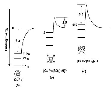
Figure 5.10. Experimentally determined electron binding energies of the neutral complex and of the complex with 3 or 4 negative sulfonate groups.
Clearly, the 6.3 eV intrinsic binding energy of the neutral complex is reduced by 5.1 eV (to 1.2 eV) by the three sulfonate groups' Coulomb repulsions. Adding the fourth sulfonate group further destabilizes the complex by another ca. 2.1 eV thus rendering the electron binding energy negative (at ca. -0.9 eV).
Let's consider the effects of a negative electron binding energy and discuss how the height of the repulsive Coulomb barrier is measured experimentally. Consider the qualitative potential energy plot shown in part (c) of Fig. 5.10. When this anion containing four sulfonate groups is subjected to laser radiation with photons of energy considerably below 3.5 eV, no photoelectrons are detected. Only as the photon energy hn approaches 3.5 eV do electrons begin to be detected. As hn reaches 3.5 eV, a rapid increase in the yield of photoelectrons is observed, so we know the height of the Coulomb barrier is ca. 3.5 eV. However, when the kinetic energies of the electrons ejected by photons of energy hn are measured, one finds the kinetic energies KE to be
KE = hn + 0.9 eV.
That is, the electrons come out with higher energy than the energy of the photon used to eject them; this is because the 4-fold charged anion lies higher in energy than the 3-fold charged anion by 0.9 eV.
Another interesting recently-stuied example from the author's lab of a multiply charged anion involves the dianion formed by coupling, in a face-to-face manner, two tetra-cyano-ethylene (TCNE) mono-anions [[223]]. In Fig. 5.11 we show the four p-type molecular orbitals one expects to obtain when two p-type orbitals (one p and one p*) from each TCNE- mono-anion are coupled to form four-centered orbitals.
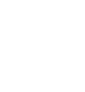 Figure 5.11. Four-centered p-type molecular orbitals (center) formed from p and p*
orbitals of two TCNE- anions (left and right).
Figure 5.11. Four-centered p-type molecular orbitals (center) formed from p and p*
orbitals of two TCNE- anions (left and right).
In each TCNE- anion, there are two electrons in the p bonding molecular orbital and one electron in the p* antibonding orbital. Thus, in the (TCNE)22- dianion, these six electrons are expected to occupy the three lowest orbitals shown in the center of Fig. 5.11. The inter-anion bonding (pR+pL) and antibonding (pR-pL) orbitals, both being doubly occupied, give rise to little net inter-ion bonding (although, of course, both of these orbitals are intra-ion bonding). The inter-ion bonding (p*R+p*L) orbital, with its two electrons, produces a net inter-ion bond order of unity. We therefore expect that there will be net inter-anion p bonding in (TCNE)22-.
In Fig. 5.12, we show the potential energy curves one obtains when two TCNE- mono-anions are brought together in a face-to-face manner to form the inter-ion p-bonded (TCNE)22-.
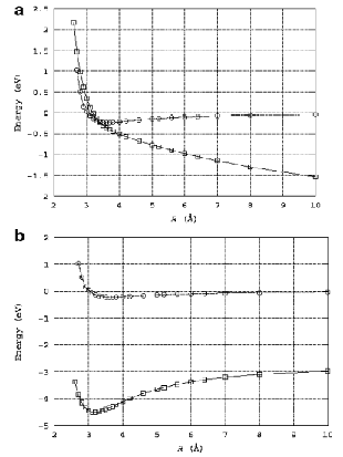
Figure 5.12. Energies of (TCNE)2- mono-anion (a, top) and (TCNE)22- (a, bottom) as functions of the distance R between the centers of the two anion's central C-C bonds. Also shown in b are these same data but with the inter-ion Coulomb repulsion removed from the dianion's energy.
From Fig. 5.12 a, we see that the two TCNE- mono-anions' p bonding is not strong enough to overcome the Coulomb repulsion pushing the two ions apart. As a result, there is no minimum in the plot of the energy of the dianion. However, if we subtract out the Coulomb repulsion and then plot the energy of the dianion as in part b of Fig. 5.12, we observe a minimum in the dianion's energy curve at ca. R = 3.2 Å. This distance, we note, is very close to the X-ray diffraction determined distance between the two TCNE- units in salts containing a variety of counter cations [[224]]. In essence by subtracting the inter-anion Coulomb repulsion, we are performing essentially the same charge-screening as do the counter ions in the solid state.
These data thus suggest the the inter-anion p bonding in (TCNE)22- has a strength of ca. 4.5 kcal mol-1 (see part b of Fig. 5.12). From part a of Fig. 5.12 we see that the (TCNE)22- dianion as an isolated species is not only geometrically unstable (i.e., there is no minimm on the energy surface) but it is also electronically unstable (i.e, it can undergo autodetachment) at inter-ion distances below ca. 3.5 Å.
IV. Special Techniques are Needed to Handle Metastable Anions
In the applications shown above involving metastable multiply charged anions, it is relatively straightforward to estimate the shape of the repulsive barrier illustrated qualitatively, for example, in Figs. 5.8 and 5.10. For example, in the SO42- case, the depth of the potential well in the absence of Coulomb repulsions can be computed by evaluating the electron binding energy E0 of the HSO4-1 anion. This E0 thus measures the intrinsic binding energy of each of the four equivalent oxygen centers in the SO42- dianion. The Coulomb repulsion, which both produces the repulsive barrier and decreases the binding energy from E0, is computed by simply evaluating e2/RLL, where RLL is the oxygen-oxygen distance in atomic units. So, for SO42-, one can use a potential as shown in Fig. 5.8 with a barrier height of e2/RLL and an energy for the metastable state of E = -E0 +e2/RLL. The energy E is positive because the Coulomb repulsion exceeds the intrinsic binding energy E0. The lifetime of such an anion can then be computed by evaluating the rate at which an electron would tunnel through such a barrier.
For some metastable anions (including both singly- and multiply-charged), it is more difficult to approximate the potential experienced by an excess electron and the barrier through which tunneling must occur may not be of the repulsive Coulomb type. For example, singly charged anions in which the excess electron occupies a molecular orbital f that possesses non-zero angular momentum have effective radial potentials as shown in Fig. 5.13.
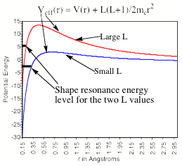
Figure 5.13. The effective radial potential experienced by an electron in an orbital having angular momentum L and attracted to the underlying molecule by a valence-range potential V(r).
For example, the p* orbital of N2- shown in Fig. 5.14 arises from two counteracting contributions to the effective radial potential Veff(r) experienced by an electron occupying it.
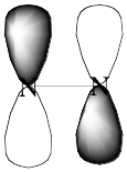
Figure 5.14. Antibonding p* orbital of N2- showing its L=2 character as viewed with respect to an origin at the midpoint of the N-N bond.
First, the two nitrogen centers exert attractive valence-range potentials on the electron in this orbital. These attractions are strongest when the excess electron is near one or both of the nuclei and decay rapidly at larger distances because the other electrons' Coulomb repulsions screen the nuclear attractions and because the polarization induced by the excess electron decays. Secondly, because the p* molecular orbital is comprised of atomic basis functions of pp, dp, etc. symmetry, it possesses non-zero angular momentum. Because the p* orbital has primary contributions from nitrogen pp basis orbitals on the two symmetry-equivalent atoms, when viewed from long distances (i.e., at large-r) the p* orbital has a dominant L = 2 angular momentum component. This character is clear in Fig. 5.14 where the p* orbital shows its centrosymmetric d-symmetry character. As a result, the excess electron also experiences (at large-r) a centrifugal radial potential L(L+1)/2m3r2 that derives from its L = 2 character.
The attractive short-range valence potentials V(r) and the centrifugal potential combine to produce a net effective potential as illustrated above in Fig. 5.13. The energy of an electron experiencing such a potential may or may not lie below the r →∞ asymptote. If the attractive potential is sufficiently strong, as it is for O2-1, the electron in the p* orbital will be bound and its energy will lie below this asymptote. On the other hand, if the attractive potential is not as strong, as is the case for the less-electronegative nitrogen atoms in N2-1, the energy of the p* orbital can lie above the asymptote. In the latter case, we speak of a metastable shape-resonance state. These states are metastable because their energies lie above the asymptote so they can decay by tunneling through the centrifugal barrier. They are called shape-resonances because their metastability arises from the angular momentum-derived shape of their repulsive centrifugal barrier.
If one had in-hand a reasonable approximation to the attractive short-range potential V(r) and if one knew the large-r L-symmetry of the orbital occupied by the excess electron, one could form Veff(r) as above. However, to compute the lifetime of the shape resonance, one has to know the energy E of this state. Unlike the situation described above for multiply charged anions, there usually is no simple way to estimate the energy of such states. Therefore, one is faced with a very difficult problem from the computational point of view. Most theoretical tools (e.g., the variational method and common perturbation methods) are designed to treat discrete bound states rather than finite-lived states such as shape resonances.
The most common and powerful tool for studying such metastable states theoretically is the stabilization method (SM). This method, pioneered by Professor Howard Taylor's group [[225]], involves embedding the system of interest (e.g., the N2-1 anion in the example we have been discussing) within a finite box in order to convert the continuum of states corresponding to N2 + e- (KE)(i.e., to an N2 molecule plus a free electron having kinetic energy KE), into discrete states that can be handled using more conventional tools of quantum mechanics. By then varying the size of the confining box, one can vary the energies of the discrete states that correspond to N2 + e- (KE) (i.e., one varies the box size to vary the kinetic energy of the orbital containing the excess electron).
To understand how this trick might work, it helps to recall how the particle-in-a-box energy levels (E = n2h2/8meL2) change as the box length L is changed. In the stabilization calculation, as the box size is varied, one eventually notices (e.g., by plotting the orbitals) that one of the N2 + e-(KE) states (i.e., one that corresponds to a certain KE-value) possesses a significant amount of valence character in addition to its large-r oscillatory continuum character that corresponds to its KE. That is, one such state has significant amplitude not only at large-r but also in the region of the two nitrogen centers. By varying the box size, one of the continuum functions has had its de Broglie wavelength (and thus its KE) varied in a manner that allows this continuum function to match (in value and derivative) the valence-range portion of the N2- wave function. It is this combination of valence-range N2- and long-range continuum (properly matched in their values and derivatives) functions that corresponds to the metastable shape-resonance state, and it is the energy where significant valence components develop that provides the stabilization estimate of the state energy.
Let us continue using N2-1 as an example for how the SM would be employed, in particular how one usually varies the box within which the anion is constrained. In the most conventional application of the SM, one uses a conventional atomic orbital basis set that would likely include s and p functions on each N atom, perhaps some polarization d functions and some conventional diffuse s and p orbitals on each N atom. These basis orbitals serve primarily to describe the motions of the 15 electrons of N2- within the usual valence regions of space.
To this basis, one would append an extra set of diffuse p-symmetry orbitals. These orbitals could be pp (and maybe dp) functions centered on each nitrogen atom, or they could be dp obitals centered at the midpoint of the N-N bond. Either choice can be used because one only needs a basis capable of describing the large-r L = 2 part of the metastable state's wave function. One usually would not add just one such function; rather several such functions, each with an orbital exponent aJ that characterizes its radial extent, would be used. Let us assume, for example, that a total of K such p functions have been used.
Next, using the conventional atomic orbital basis as well as the K extra p basis functions, one carries out a calculation (most often a variational calculation in which one computes many energy levels, but it could be an EOM calculation on N2 in which one evaluates several EA values) on the N2-1 anion. In this calculation, one tabulates the energies of many (say M) of the electronic states of N2-1. One then scales the orbital exponents {aJ} of the K extra p basis orbitals by a factor h: aJ h aJ and repeats the calculation of the energies of the M lowest energies of N2-1. This scaling causes the extra p basis orbitals to contract radially (if h > 1) or to expand radially (if h < 1). It is this basis orbital expansion and contraction that produces what is the practical implementation of the expansion and contraction of the box discussed above. That is, one does not employ a box directly; instead, one varies the radial extent of the more diffuse basis orbitals to simulate the box variation.
If the conventional orbital basis is adequate, one finds that the extra p orbitals, whose exponents are being scaled, do not affect appreciably the energy of the neutral N2 molecule. This can be probed by plotting the N2 energy as a function of the scaling parameter h; if the energy varies little with h, the conventional basis is adequate.
In contrast to plots of the neutral N2 energy vs. h, plots of the energies of the M N2-1 anion states (or, equivalently, plots of the energies of these anion states relative to the energy of the neutral) show significant h-dependence as Fig. 5.15 illustrates.
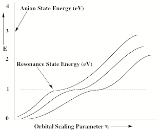 Figure 5.15. Plots of the energies of several anion states vs. the orbital scaling
parameter h. Note the avoided crossing of state energies near 1 eV.
Figure 5.15. Plots of the energies of several anion states vs. the orbital scaling
parameter h. Note the avoided crossing of state energies near 1 eV.
What does such a stabilization plot tell us and what do the various branches of the plot mean? First, one should notice that each of the plots of the energy of an anion state (relative to the neutral molecule's energy, which is independent of h) grows with increasing h. This h-dependence arises from the h-scaling of the extra diffuse p basis orbitals. Because most of the amplitude of such basis orbitals lies outside the valence region, the kinetic energy is the dominant contributor to such orbitals' energies. Because h enters into each Gaussian basis orbital as exp(-ha r2), and because the kinetic energy operator involves the second derivative with respect to r, the kinetic energies of orbitals dominated by the h-scaled diffuse p basis functions vary as h2. It is this quadratic growth with h that is shown in Fig 5.15.
For small h, all of the p diffuse basis functions have their amplitudes concentrated at large-r and have low kinetic energy. As h grows, these functions become more radially compact and their kinetic energies grow. For example, note the three lowest energies shown above in Fig. 5.15 increasing from near zero as h grows. As h further increases, one reaches a point at which two of the anion-state energies in Fig. 5.15 undergo an avoided crossing. At this h-value, if one examines the nature of the two wave functions whose energies avoid one another, one finds that one of them contains substantial amounts of both valence and extra-diffuse p-function character. Just to the left of the avoided crossing, the lower-energy state contains predominantly extra diffuse p-orbital character, while the higher-energy state contains largely valence p* orbital character. In Fig. 5.15, other avoided crossings occur at higher h-values. For each such crossing, the situation is similar to what I just said. The lower-energy eigenfunction to the left of the avoided crossing contains predominantly extra diffuse p orbital character, while the higher-energy state contains largely valence p* orbital character.
At any of the special values of h where two states nearly cross, the kinetic energy of the continuum state (as well as its radial size and de Broglie wavelength) are appropriate to connect properly with the valence-region state. By connect properly I mean that the two states have wave function amplitudes, phases, and slopes that match. It is such boundary condition matching of valence-range and long-range character in the wave function that the stabilization method achieves. So, at such a special h-value, one can achieve a description of the shape-resonance state that correctly describes this state both in the valence region and in the large-r region. Only by tuning the energy of the large-r states using the h-scaling can one obtain this proper boundary condition matching.
If one attempts to study such metastable anion states without carrying out such a stabilization study, one is doomed to failure, even if one employs an extremely large and flexible set of diffuse basis functions. In fact, in such a large-basis calculation, one will certainly obtain a large number of anion states with energies lying above that of the neutral, but one will not be able to select from these states the one that is the true resonance state. Most of the states will simply be states describing an N2 molecule with an excess electron at large-r and low KE, but, in the absence of the SM, none will offer a proper description of the metastable state.
In summary, by carrying out a series of anion-state energy calculations for several states and plotting their energies vs. h, one obtains a stabilization graph. By examining this graph and looking for avoided crossings, one can identify the energies at which metastable resonances occur. It is absolutely critical to identify these resonance energies if one wishes to probe metastable anions. It is also possible [[226]] to use the shapes (i.e., the magnitude of the energy splitting between the two states and the slopes of the two avoiding curves) of the avoided crossings in a stabilization graph to compute the lifetimes of the metastable states. Basically, the larger the avoided crossing energy splitting dE between the two states, the shorter is the lifetime t of the resonance state and t ≈ h/dE.
The above examples illustrate how one faces additional complications when dealing with anions that are not electronically stable (i.e., that can spontaneously eject an electron). These difficulties should be kept in mind whenever one attempts to study such anions using conventional quantum chemistry tools. The most important thing to remember is that one should not simply proceed to try to study such metastable anions using conventional atomic orbital bases (even if diffuse functions are included). Unless one uses a stabilization-type method to determine the proper energy of the resonance, one cannot be assured of having the correct energy. An arbitrarily chosen basis, even with diffuse functions included, will yield but an arbitrary energy for the metastable anion rather than the correct resonance energy. One must properly couple the valence component of the wave function to the large-r component (as the stabilization method does) to achieve the correct results.
Before closing this Section dealing with the special techniques that must be used to handle metastable states, it is useful to discuss an approximation to the stabilization method that derives from Professor Sigrid Peyerimhoff's lab and that has proven useful in many cases. It should be clear from the above description of how the SM is implemented that this can be a very tedious approach that requires one to compute the energies of many states of the anion (or multiply-charged anion) to properly identify and characterize the desired metastable state. An approach that is more direct involves what is called the charge-stabilization trick. I will illustrate this approach using the SO42- dianion as an example.
As noted earlier, SO42- is metastable with respect to SO4- + e-, so, as noted above it is futile to attempt a straightforward (e.g., variational) calculation of the energy of SO42-. However, consider what would happen if one were to artificially enhance the nuclear charge on the sulfur nucleus from 16 by a small amount, dq. In effect, one would be mutating (as dq → 1) SO42- toward the isoelectronic mono-anion ClO4-, which has a positive electron binding energy. So, in this approach, one carries out a series of calculations on the dianion-anion energy separation as a function of dq using only those values of dq that are large enough to render the dianion electronically stable. One then plots these energy-separation data vs. dq and extrapolates to dq → 0 to obtain an estimate of the (negative) electron binding energy of the original species (SO42- in this example). In Fig. 5.16, we see an example [21] from the author's lab of such a charge-stabilization plot for the SO42- dianion.
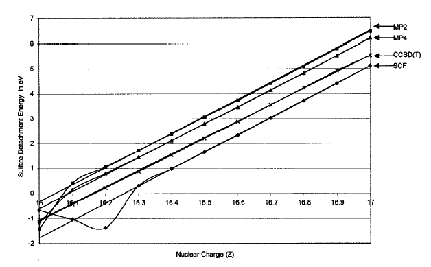
Figure 5.16. Charge-stabilization plot of the dianion-anion energy difference vs. the total nuclear charge Z on the sulfur atom performed at various levels of theory.
From these plots (at various levels of theory), one can extrapolate to dq → 0 to predict the energy of SO42- relative to SO4-. The highest-level data (i.e., the coupled-cluster data labeled CCSD(T)) predicts that SO42- is unstable by ca. 0.9 eV. I should note that one is not required to modify the sulfur's nuclear charge; one could, alternatively, modify the charges of the four oxygen nuclei or one could modify the charges of the oxygen and sulfur nuclei. One is, however, required to make these modificactions in a way that preserves the spatial symmetry of the Hamiltonian; this means, one must alter all of the oxygen nuclear changes by the same amount, for example.
This charge-stabilization technique works because an increase in the nuclear charge(s) introduces into the electronic Hamiltonian a perturbation potential
V= Sj (-dq e2/rj)
where rj is the distance of the jth electron to the nucleus whose charge in incremented by dq. Because this potential is stabilizing (i.e., negative) in regions of space near the nucleus, it tends to lower the energies of states having high electron density in the valence region relative to states with high density in the large-r region. This causes the perturbation to differentially stabilize valence-localized electron-attached states and thus to render positive the electron binding energies of such states. Once these states have positive binding energies, they can be treated reliably using conventional quantum chemistry tools such as were discussed in Chapter 2.
I should note that Professor Lenz Cederbaum's group has used similar [[227]] extrapolation type technquies for determining energies of metastable states with great success. They have, I believe, carried out more theoretical studies on multiply charged anions than any other group and have recently found a reasonably small electronically stable triply charged anion whose structure is shown in Fig. 5.17.
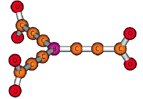
Figure 5.17. Structure of the triply charged anion studied by the Cederbaum group.
This species has been predicted [[228]] to be vertically electronically stable with respect to electron loss by ca. 0.3 eV. The reason I mention that this is a reasonably small tri-anion is that it is especially challenging to find small highly charged anions because the internal Coulomb repulsions in such species is especially high.
Let us finish this Chapter with one more example of using the charge-stabilization method to study metastable electronic states. In a recent joint experimental and theoretical re-investigation [[229]] of O2 and O2-, our group needed to compute the energies of several low-energy states of the O2- anion over a wide range of internuclear separations. Although, as is widely known, O2 has a positive adiabatic electron affinity, the energies of the ground (X2Pg) and low-lying (a4Su- and A2Pu) states relative to the X3Sg- ground state of neutral O2 vary strongly with bond length R. In Fig. 5.18 we display the neutral (determined from experimental data) and anion (from our calculations) energy curves resulting from this collaborative effort.
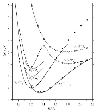
Figure 5.18. Potential energy curves of low-energy states of O2 and O2-.
At bond lengths where one or more anion state energy lies above the energy of the ground state of the neutral, we needed to perform charge stabilization extrapolations to obtain the data points shown in Fig. 5.18. An example of a charge stabilization used in this project is shown in Fig. 5.19 where we see the extrapolations needed to locate the energies of three anion states at R = 1.313 Å.
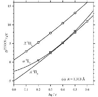
Figure 5.19. Charge stabilization plot showing the energies of three anion states relative to the O2 neutral's ground state as a function of the incremental charge on each oxygen nucleus.
Notice that the X2Pg state's energy extrapolates to a positive value meaning it is bound relative to the ground state of neutral O2 as shown in Fig. 5.18 where the potential curves appear. Of course, we did not have to carry out a charge stabilization calculation for this state of the anion; we did so simply to illustrate that, when applied to stable states, this method still yields the correct answer. The two other anion states of 4Su and 2Pu symmetry are not electronically stable, so the charge stabilization extrapolation shown in Fig. 5.19 is necessary for them. The extrapolated values of their energies obtained from Fig. 5.19 are then used as two of the data points (at R = 1.313 Å) in Fig. 5.18.
Chapter 6. Cluster Anions
In this Chapter, we will focus on clusters comprised either of a conventional anion surrounded by one or more solvent molecules, or an anion that can best be viewed as a cluster of atoms or molecules to which an electron has been added. Of course, one can imagine a nearly limitless number of clusters containing three, four, five, and more atoms to which electrons might bind. So, it is impossible, and in my mind fruitless, to attempt to survey or even categorize all possible such species. Instead, I will attempt to introduce the reader to a few broad classes of cluster anions that have received considerable experimental and theoretical study. The web pages of Professor Kit Bowen, Professor Lai-Sheng Wang and Professor Alex Boldyrev offer many examples of very interesting cluster anions constructed from many different atoms. The web pages of Professor Ken Jordan, Professor Mark Johnson, Professor Dan Neumark, Professor Jim Coe, Professor Kit Bowen, and Professor Carl Lineberger offer a wealth of information about cluster anions comprised of an anion or electron surrounded by solvent molecules.
I. Anions that are Solvated
An example of a solved anion is provided by Cl-(H2O)n, a typical solvation structure of which is qualitatively illustrated in Fig. 6.1.
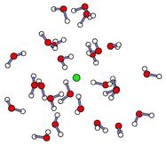
Figure 6.1. A depiction of a chloride anion surrounded by 25 H2O molecules.
The main characteristics of such solvated cluster anions that one should be aware of are that:
- The electron binding energy of the cluster anion is larger than that of the isolated anion (e.g., Cl-(H2O)25 binds its excess electron more strongly that does Cl-) because of the significant differential solvation energy of the charged species.
- There is usually a very large geometrical reorganization of the surrounding solvent molecules that accompanies electron detachment (e.g., the H2O molecules most often have the positive ends of their dipoles directed toward the Cl-ion, but for the neutral Cl, the H2O molecules' dipoles are less oriented). This fact makes it difficult, if not essentially impossible to determine adiabatic electron binding energies using photodetachment probes because the Franck-Condon factors connecting the neutral and anion structures are extremely small.
When studying this kind of clusters with a small number of solvent molecules present, it is found that the most stable geometry (in an energy or free-energy sense) does not always involve the anion being completely surrounded by solvent molecules. Instead, the anion may find it energetically and entropically favorable to sit on the surface of a cluster of solvent molecules. An example of such a case (that of I2- surrounded by a few solvent CO2 molecules) from Profesor Carl Lineberger's lab is shown in Fig. 6.2.
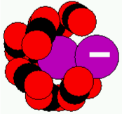 Figure 6.2. Representative structure of I2- anion solvated by CO2 molecules.
This preference to place the anion not fully interior to the solvent molecules, which tends to occur for small numbers of solvent molecules, arises from two effects:
- To surround the anion by a shell of solvent molecules, one may have to arrange the solvents such that their dipoles, while directed toward the anion, are in highly unfavorable orientations with respect to one another. That is, the dipoles are directed toward one another. This certainly is the case in the Cl-(H2O)25cluster shown in Fig. 6.1.
- Placing the anion in the interior of a cluster disrupts more inter-solvent attractive interactions (e.g., hydrogen bonds in the water clusters; Van der Waals attractions in the CO2clusters) than when the anion is placed on the surface of the solvent cluster and the solvent is allowed to retain the network of attractive interactions that optimally stabilize it.
Thus, it is important to be aware that one may be dealing with surface-localized anions rather than internally solvated anions, especially when small cluster sizes are involved.
A very interesting example from Professor Pavel Jungwirth's lab of how various ions may prefer to reside on the surface rather than in the interior is offered in Fig. 6.3 where we show the ions' spatial distributions in aqueous H+/Cl-, H+/Br-, Na+/OH-, and Na+/Cl- solutions near an air-water interface. These species were studied [[230]] using molecular dynamics simulations to obtain these data. On the right side of Fig. 6.3 are shown plots of the probability densities for finding these ions (labeled with the same color scheme) as a function of distance with z = 15 Å corresponding to the air-water interface and z = 0 Å being inside the liquid.
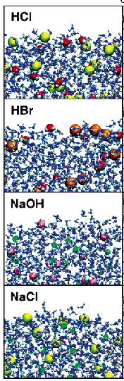
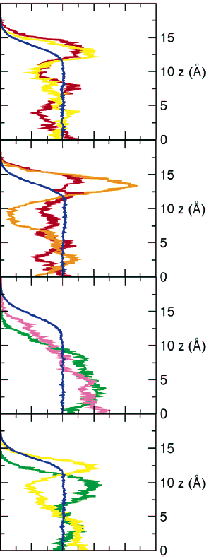
Figure 6.3 Depictions of typical spatial distributions of water molecules (blue) and of H+ (red), OH- (pink), Na+ (green), Cl- (yellow), and Br- (orange) ions near the air (top)-water (below) interface.
These plots clearly show that the ions do not all prefer to be isotropically distributed within the aqueous sample; some are more localized near the interface while others spend more time deeper within the liquid.
Another example of how the solvation environment of an anion surrounded by a modest number of solvent molecules can be surprising is provided by data from Professor Mark Johnson's lab [[231]] in Fig. 6.4. Clearly, these structures make sense in that they involve water molecules with their H atoms directed toward the anionic center, but they differ in how many water-water hydrogen bonds they possess. Certainly, they are not structures that one could easily guess if one assumed that ions are isotropically surrounded by solvent molecules.
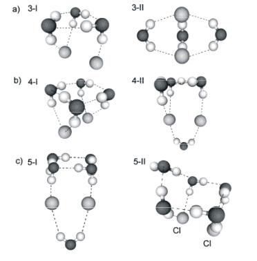
Figure 6.4 Low-energy structures of I2-(H2O)n with n = 3, 4, and 5 [231].
Another example of such anisotropic solvation is provided by the Johnson group's data [[232]] on NO-(H2O)3. In Fig. 6.5, we see there are several local minima on the ground-state energy surface that differ in how the NO- anion's nitrogen and oxygen atoms interact with the water molecules. These different interactions produce different kinds of O-H vibrations in the infrared spectrum, which the Johnson group has used, in connection with ab initio calculations, to identify these structures.
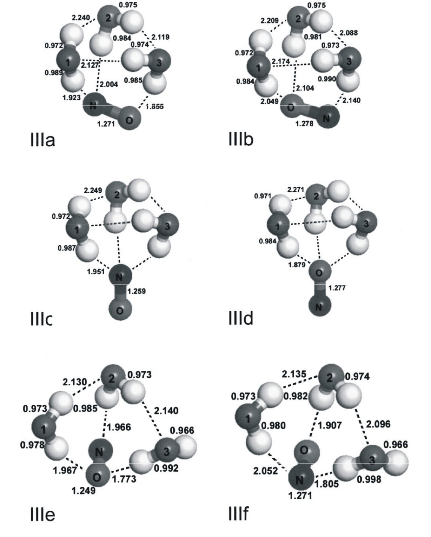
Figure 6.5 Low-energy structures of NO-((H2O)3 varying in how many and what types of hydrogen bonds are present [232].
An example of how the solvation of an anion tends to become more isotropic as the number of solvent molecules grows is shown in Fig. 6.6 where we see structures of I2-(OCS)n with n = 5, 11, and 17 taken from Professor Carl Linebergers' lab [[233]].
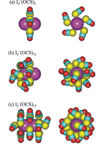
Figure 6.6. Low-energy structures of I2-(OCS)n for n = 5, 11, and 17 [233].
An especially illustrative example of how the nature of the electronic states can change when an anion is solvated is provided by Professor Steve Bradforth's [[234]] study of electronic excitations of I- in water. The experimental spectroscopic data gathered by Bradforth's lab is consistent with the theoretical picture they also developed in which an electronic transition occurs between two very different states of the anion cluster. In the initial state (i.e., prior to photoexcitation), the electron resides in an orbital localized on the I- center; this orbital is shown in Fig. 6.7 for a case when six water molecules solvate the anion.
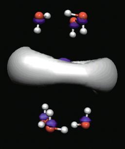
Figure 6.7 Orbital of I- (center) surrounded by six water molecules
In Fig. 6.8 we show the orbital into which the electron is promoted upon excitation. The electronic transition to this particular orbital is termed a charge-transfer-to-solvent (CTTS) transition because the electron is promoted from the iodine to an orbital in which it is bound not to the iodine center but by the electrostatic potential of the cluster of solvent molecules.
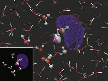 Figure 6.8 Charge transfer to solvent orbital resulting from photoexcitation of the
I-.
Figure 6.8 Charge transfer to solvent orbital resulting from photoexcitation of the
I-.
The lesson that this example teaches is that the excess electron can be bound by a site of high electron affinity such as the I atom, but it can also be bound by the surrounding solvent molecules. It also illustrates that electronic transitions indeed do occur between the solvated-anion state and the CTTS state.
Another good example of the anisotropic solvation structures arising in solvated anions is seen in early work from this author's lab [[235]] on the geometries and energetics of small NO2-(H2O)n clusters. In Fig. 6.9, we show the radial and angular distributions of H2O molecules around the NO2- anion determined using Monte-Carlo simulations at T = 300 K. The radial variable R is defined as the distance from the nitrogen atom in NO2- to a water molecule's oxygen atom. The variable q is the angle between the vector connecting the NO2- nitrogen to any water's oxygen and the C2 axis of the NO2- with q = 0 corresponding to a water oxygen atom nearer the nitrogen of NO2-.
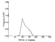
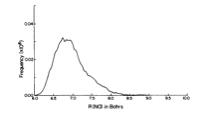
n=3
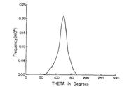
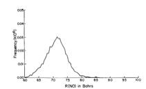
n=5
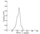
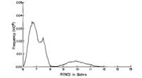
n=6
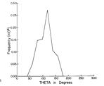
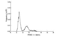
n=9
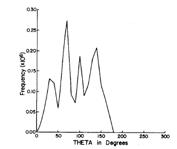
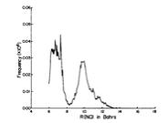
n=15
Figure 6.9. Angular (theta) and radial(R) distributions for n H2O molecules relative to a central NO2- anion at T = 300 K [235].
We note that the angular distribution of water molecules about the NO2- anion does not approach the sin(q) distribution that characterizes an isotropic distribution until ca. 9-15 water molecules are present. For the smaller clusters in particular, angles between q = 50 and 150 seem to be preferred. Hence, it appears that the first solvation shell is not angularly complete (i.e., water molecules seen at all angles) until n = 9-15. These clusters thus consist of a nitrite anion with water molecules bound to it with the waters located primarily at angles q > 50 .
The radial distribution functions indicate that a second solvation shell begins to form at n = 6 (i.e., note the second peak near 10 bohrs), and a third shell may begin at n = 9. Clearly, by the time one has 15 H2O molecules present, there are at least two distinct radial distributions. This suggests that second and third solvation shells may begin to form even before the first shell is angularly filled.
The NO2-..H2O attractions, which act to place the water molecules near the oxygen atoms of NO2- (where the negative charge is localized) with their dipoles oriented toward the nitrite, and the H2O...H2O dipole-dipole interactions, which prefer to have the water molecules in the same q hemisphere rather than opposite one another where their dipoles repel, combine to produce the highly anisotropic q-distributions and the unusually non-spherical cluster geometries observed above.
The examples we have discussed show that solvated anions are not as simple as one is taught in introductory chemistry classes, especially when they contain small numbers of solvent molecules or when the anions reside on a surface or near an iterface. The competition between anion-solvent and solvent-solvent interaction potentials often produces cluster anions that have angularly anisotropic shapes and unusual radial distributions.
II. Clusters With an Electron Attached
A different kind of cluster anion arises when one attaches an excess electron to a cluster of solvent molecules rather than when one embeds an anion among these solvent molecules. Two examples are provided by the neutral water tetramer and its anion shown in Fig. 6.10 and the CTTS state of the I-(H2O)n cluster discussed earlier.
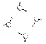
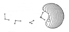
Figure 6.10. Most energetically stable structure of (H2O)4 neutral (above) and of the (H2O)4- anion (below). The orbital in which the excess electron resides is also show below.
One clearly notes the very large geometrical reorganization that accompanies electron attachment (i.e., in moving from the neutral to the anion). In the neutral water tetramer, the network of hydrogen bonds among neighboring water molecules plays a dominant role in determining the lowest-energy structure, which is square-like. However, this structure does not present to an excess electron a very attractive potential to which it can bind. In contrast, the quasi-linear geometry shown in the bottom part of Fig. 6.10 generates a large dipole potential to which the excess electron can bind more strongly. Of course, the latter geometry is not the most stable structure in the absence of the excess electron because it has fewer internal hydrogen bonds than the quasi-square structure. Again, we see an example of how the competition between solvent-solvent attractions and electron-solvent attractions give rise to vastly different neutral and anion structures.
These large anion-neutral geometry differences make it very difficult to form the dipole-bound anions of such clusters from the corresponding neutrals by electron attachment because it is very rare that the neutral's equilibrium thermal motions cause it to sample the extended geometry where dipole-binding electron attachment can occur. In addition, as noted earlier, these large geometry differences cause difficulties in analyzing the photoelectron spectra of the corresponding anions because of the very broad Franck-Condon progressions that accompany such extreme geometry changes.
It is not true, however, that the optimal geometry of the cluster anion is always very different from the structure of the neutral parent. For example, in the water dimer shown in Fig. 6.11, the anion and the neutral both adopt geometries with one hydrogen bond connecting the two water molecules.
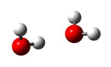
Figure 6.11 Geometry of the water dimmer anion, which is very similar to that of the neutral water dimmer.
Another factor that tends to complicate matters is that anions formed by attaching an electron to a molecular cluster often have more than one geometry that correspond to true local minima on the electronic ground-state surface or which are frequently populated in laboratory measurements. For example, two structures corresponding to local minima of (H2O)3- and two minima of (H2O)4- are shown in Fig. 6.12.
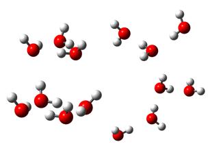
Figure 6.12. Two low-energy local-minimum structures of water trimer anion (top) and water tetramer anion (below).
In such cases, experimental samples of the anion may contain both structures in abundances that will usually depend on their relative energies and upon how the anion sample was prepared. If the pairs of structures have considerably different electron binding energies or vibrational frequencies, then photoelectron or infrared spectroscopy can be used to probe the relative abundances of the two structures if one knows which spectral features to assign to which structure (which is where good theoretical simulations prove very useful).
The study of water cluster anions, viewed as a probe of electrons solvated by water molecules, has developed into an area that has attracted many of the best people in the field and has produced a very interesting body of work that I will now outline. Several years ago, a group [[236]] involving Professor Jim Coe and Professor Kit Bowen measured the electron detachment energies of a wide range of size-selected (H2O)n- cluster anions. One of their goals was to explore how the behavior of such anions converged (or did not) to the behavior of solvated electrons in bulk water.
With this in mind, Coe and Bowen plotted the electron binding energies vs. n-1/3 as shown in Fig. 6.14 (n-1/3 being proportional to the cluster radius if the clusters were pseudo-spherical). They did not know the structures of the cluster anions, but they were testing a hypothesis that the clusters might bind the excess electron within a cavity as in bulk water. The group of Professor Uzi Landman had shown [[237]] that electrons trapped within a spherical dielectric cavity would have binding energies that vary inversely with the cavity radius. This dependence can be qualitatively understood by considering the simple cavity model shown in Fig. 6.13.
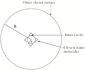
Figure 6.13. Ideal spherical cluster model showing inner cavity of radius r and cluster of radius R.
If one assumes the cavity is filled uniformly with n molecules each having a polarizability a from a radial distance r out to radius R and that an excess electron resides within the inner cavity, one can write the charge-polarization stabilization energy for this electron interacting with the n molecules as:
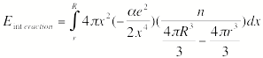 .
.
Here,
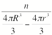
is the number of water molecules per unit volume which we will denote r, (-ae2/2x4) is the interaction energy of an electron a distance x from a molecule with polarizability a, and 4px2 is the radial volume element. This interaction energy integral can be reduced to
![]() .
.
In the R >> r limit, R is proportional to n1/3, so Einteraction will scale as n-1/3; this kind of argument is the basis for expecting the electron binding energies to scale as n-1/3. The data obtained in ref. 236 is shown plotted vs n-1/3 in Fig. 6.14.
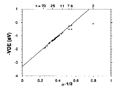
Figure 6.14. Plot of the (vertical) photodetachment energies of size selected water cluster anions.
Notice that most of the data lie on a straight line when plotted vs. n-1/3 and that this line extrapolates (n →∞) to ca. 3.2 eV, which, as Coe points out [[238]], is the value appropriate to an electron in bulk water. These observations suggested that these water cluster anions exist in sphere-like shapes with the excess electron bound near the center of the sphere. However, Fig. 6.14 also contains a few data points for n = 7 and smaller that seem to correspond to lower electron binding energies and to lie on a line of smaller slope suggesting that smaller cluster anions may be different than the larger species. In fact, for these smaller cluster sizes, there are two data points for a given cluster size, suggesting that more than one kind (i.e., isomer) of cluster may exist for a given size.
A later study of size-selected water cluster anions by Professor Dan Neumark's group [[239]] produced data (and overviewed earlier data by others) on the electron detachment energies of water cluster anions that are summarized in Fig. 6.15. The data labeled Kim et. al. [[240]] came from an earlier experimental study from Professor Mark Johnson's lab. Those labeled internal calculated and surface calculated came from Professor Uzi Landman's quantum dynamics simulations [237]. The Neumark group then multiplicatively scaled the latter values and noticed these scaled energies agreed reasonably well with their experimental data.
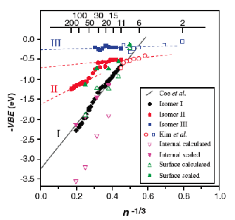
Figure 6.15. Plots of vertical electron detachment energies vs. n-1/3 showing clusters of a given size can exist in more than one form.
The data shown in Fig. 6.15 suggest that, for a given cluster size, indeed there can be more than one isomer and the various isomers can have significantly different electron binding energies. The data for the isomer labeled I seem to extrapolate to ca. 3.2 eV, the value for electrons in bulk water, so it would appear the ions belonging to category I hold the excess electron on their interiors as in the bulk. Moreover, there seem to be at least two other isomer categories (II and III) that bind the excess electron less tightly than does the type-I isomer for a given cluster size. It was surmised that one or both of categories II and III have structures that bind the excess electron on the surface of the cluster because the simulations of Landman had shown that such surface-bound species had smaller electron binding energies.
Further evidence from Professor Dan Neumark's group [239] comes in the form of pump-probe experiments in which they pumped size-selected water cluster anions from their electronic ground state to an excited electronic state and followed the relaxation back to the ground state. The lifetimes of the excited state (i.e. how long the excited state took to decay back to the ground state) were determined for ions from category I (termed internal) and category II (termed surface) and plotted vs n-1 as shown in Fig. 6.16. The group of Professor Ahmed Zewail performed similar time-resolved experiments and obtained similar results [[241]].
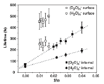
Figure 6.16. Lifetimes for return to the ground state from an electronically excited state for size-selected clusters of type I (internal) and type II (surface) plotted vs. n-1.
A key observation on these relaxation rate data is that the rates for the internal clusters extrapolate (at n →∞) to ca. 50 fs which happens to be the relaxation time observed [[242]] for electrons in bulk water (i.e. for relaxing from the excited p-type state back to the s-type ground state). So, much of the vertical detachment energy and excited-state relaxation data seem to point to the type-I clusters binding the excess electron on the interior.
However, more recent quantum dynamical simulations from Professor Peter Rossky's group [[243]] on water cluster anions containing from 20 to 200 water molecules suggested that the exces electron is more likely to be bound on or near the surface at least for clusters of size n < 100. In Fig. 6.17 we display a typical structrure for (H2O)45- obtained in the Rossky-group simulations showing the excess electron in its ground and lowest-excited electronic states, both of which are clearly surface-bound.
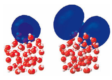
Figure 6.17. Ground (left) and excited (right)- state orbitals for the excess electron in the (H2O)45- cluster anion.
Moreover, Rossky pointed out that Professor Abe Nitzan's group [[244]] had earlier shown that both interior and surface states can display electron binding energies that scale as n-1/3, so it may not be possible to use this scaling feature to assign the geometry of cluster classes I, II, and III.
In addition, Professo Ken Jordan's group has carried out numerous simulations [[245]] on small to medium size cluster anions in which the Drude model discussed in Chapter 4 was used to handle the electronic structure aspect, and energy-minimization and Monte-Carlo sampling were used to identify low-energy (and low-free energy) geometrical structures. As illustrated in Fig. 6.18 for clusters containing 12 through 24 water molecules, they found low-energy structures in which the excess electron is surface-bound and equally low-energy structures with the electron interior-bound. Moreover, they noted that, in some cases, the surface-bound anion has a larger vertical detachment energy than does the corresponding (i.e, for the same cluster size) interior-bound anion, while, for other cluster sizes, the interior-bound anion has the larger detachment energy. They thus called into question the idea that one can distinguish among structural isomers by using the magnitude of the electron binding energy (e.g., assuming all anions belonging to category I in Fig. 6.15 are interior-bound).
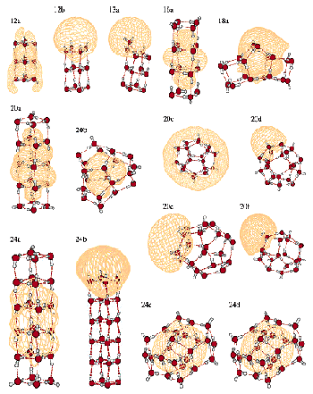
Figure 6.18. Low-energy structures of (H2O)n- with n between 12 and 24 showing selected interior-bound and surface-bound states.
So, the trends observed in the early Coe and Bowen data and again in more recent Neumark, Zewail, and Johnson data seem to point toward ions in category I being interior-bound. The existence of one or more distinct classes (II and III) having smaller electron binding energies (and distinct relaxation times) then points toward these classes being surface-bound. However, the simulations of Rossky and Nitzan's showing that n-1/3 scaling can apply to surface and interior ions, as well as Jordan's observations suggest that it may not be at all clear (yet) that class-I ions are interior-bound while class-II and class-III are surface-bound.
Another interesting feature of the story surrounding water cluster anions is how the water molecules nearest the excess electron are geometrically arranged. By using a very clever action-spectroscopy technique, Professor Mark Johnson's lab [[246]] has been able to probe the infrared (IR) spectra of water cluster anions. In particular, by focusing on the IR spectra in the frequency range where O-H stretching and bending vibrations absorb, they have been able to identify features that distinguish among water molecules' hydrogen bonding characters.
These workers form mixed clusters such as (H2O)n-Arm, subject them to IR radiation and subsequently monitor the disappearance of ions having the parent ion's charge to mass ratio or the appearance of ions that have lost one or more Ar atom (H2O)n-Arm-k . The key to this spectroscopy is that the IR energy, although, initially absorbed by, for example, a symmetric or asymmetric O-H stretching or HOH bending mode, is subsequently converted to lower-frequency modes that couple into the cluster-Ar motion and eject one or more Ar atoms. Thus, using the highly sensitive mass-dependent signal they produced a wonderful way to monitor IR absorption.
By measuring the IR spectra of various small mass-selected water cluster anions, the Johnson group has been able to identify a spectral feature that they call the double-acceptor (AA) feature and that is common to all small water cluster anions. Using theoretical contributions from Professor Ken Jordan's group, Johnson has been able to identify this feature as involving a water molecule to which the excess electron is most closely bound and which is involved, as an acceptor, in hydrogen bonds with two other water molecules. In Fig. 6.19 we see an example of the orbital holding the excess electron as well as of the AA water molecule on the left.
 Figure 6. 19. Water tetramer anion with the orbital holding the excess electron shown.
Also, on the left is the double-acceptor (AA) water molecule.
Figure 6. 19. Water tetramer anion with the orbital holding the excess electron shown.
Also, on the left is the double-acceptor (AA) water molecule.
In all of the clusters that Johnson has studied using the IR action spectrocopic tool, they have seen clear signatures of the AA water molecule. It is believed that this AA structural motif, which Professor Kwang Kim's group originally proposed [[247]], is key to binding the excess electron, perhaps in all water cluster anions.
Professor John Herbert and Professor Martin Head-Gordon showed [[248]] how the excess electron gives rise to the characteristic shifts in the O-H stretching frequencies that the Johnson group sees in the kind of small to medium size water cluster anions they study. In Fig. 6.20 we see the surface-bound electron's orbital (a, b, and e) in the (H2O)6- anion, and, in c and d we see O-H s* antibonding orbitals on one of the water molecules in this cluster.
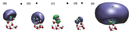
Figure 6. 20. Surface bound electron's orbital (a, b, e) and O-H s* orbital in the (H2O)6-.
Herbert and Head-Gordon suggest that mixing of the AA-localized orbital holding the excess electron with the O-H s* orbital on the AA water molecule is what gives rise to the specific shift in the IR absorption frequency for this AA molecule.
Another example [[249]] of an anion comprised of an excess electron attached to a molecular cluster is offered in Fig. 6.21 from Professor Piotr Skurski's group where urea molecules are used to bind the electron.
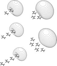
Figure 6.21. Urea dimer through pentamer anions, showing the orbital in which the excess electron resides.
In this case, both the linear chain (left) and ribbon (right) geometries of the neutral urea ((NH2)2C=O)n clusters are geometrically stable and have large dipole moments. These moments create a substantial electrostatic potential to which the excess electron can bind. Analogous situations arise in (HF)n, (HCN)n and other clusters, some of which were discussed earlier.
We thus see that closed-shell polar molecules often form closed structures containing internal hydrogen-bond (or other intermolecular interaction based) networks in their neutrals, but more spatially extended (e.g., quasi-linear for the water clusters shown earlier) structures with large dipole moments for their anions. However, these same species also form another type of anion structure (i.e., a so-called solvated-electron (SE) structure) that is illustrated in Fig. 6.22 for the urea case from Professor Piotr Skurski's lab [[250]].
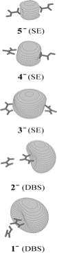 Figure 6.22. Linear dipole-bound (1- and 2-) and solvated-electron (3-, 4-, and 5-) structures of the urea dimer anion.
In structures 2- and 3-, respectively, the urea monomers are arranged to form a highly polar dipole-bound anion and a solvated-electron cluster in which the dipoles are directed inward. The relative energies of these two species are indicted by their vertical (energy) placements and are determined by the relative magnitudes of the electron-dipole attraction and the dipole-dipole repulsion with the latter disfavoring the SE species.
Structures 4- and 5- are also solvated-electron structures but with one or both urea building blocks in their zwitterion tautomeric state, respectively. Notice that, in all of the solvated-electron structures, the dipoles of the urea molecules are directed inward toward the excess electron in an orientation that would be quite energetically unfavorable if the excess electron were not present. That is, such structures are not stable for the corresponding neutral species. This same situation arises in electrons that are solvated in bulk water or ammonia where the solvent molecules closest to the excess electron have their dipoles strongly oriented inward. Once the solvated electron migrates to a neighboring group of solvent molecules (or is photoexcited and caused to escape its initial cavity), the solvent molecules in the initial cavity will react and undergo significant geometrical rearrangements to achieve a new energetically stable structure.
In Fig. 6.23 we show several structures of anions formed by water clusters that bind an electron and that are also solvated by various numbers of Ar atoms. These species have been studied by Professor Ken Jordan's group [[251]].
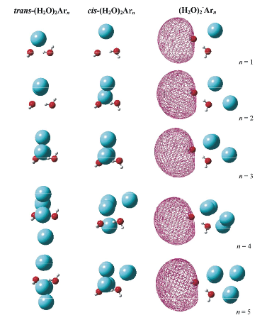
Figure 6.23 Structures of (H2O)2-Arn n = 1, 2, ... 5 [251].
Also shown in Fig. 6.23 is the orbital that the excess electron resides in. Notice that all of the Ar atoms solvate the side of the cluster that is opposite the bound electron. If the Ar atoms were to instead reside where the excess electron is shown, their presence would block the electron from attaching to this location.
III. Clusters Can be Used to Probe Chemical Reactions
As the examples just discussed illustrate, at times, even relatively simple cluster anions can be more complicated than one might think. Moreover, a cluster anion can sometimes have a geometry that is similar to that of a transition state on the neutral-molecule's reaction surface. For example, consider that one were studying a complex in which an anion of a strong acid is involved in a hydrogen bond with a weaker acid such as Cl-···H-I. The H-I bond length in this complex is elongated compared to what it is in isolated HI, and the Cl-···H distance is much longer than in HCl. In fact, the H-I and Cl-···H distances are rather close to those associated with the transition state for the reaction of neutral Cl with H-I to produce Cl-H + I. So, by using the Cl-···H-I complex as a precursor, one can, by photodetaching the excess electron, place the resulting neutral Cl···H-I complex at a geometry that is near its transition state.
An example from Professors Dan Neumark's and Carl Lineberger's labs is shown in Fig. 6.24 for a case that illustrates how anion clusters are used to probe chemical reactions of the daughter neutral species.
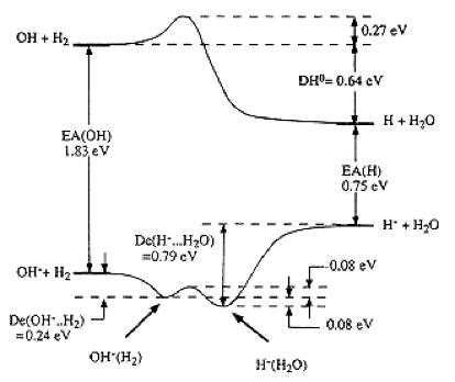
Figure 6.24. Energy profile of the part of (H3O)- and (H3O) ground-state surfaces.
Notice how the geometry of the OH-···H2 complex that lies 0.24 eV below OH- + H2 is shown as being near that for the transition state on the neutral OH + H2→ OH2 + H surface at the top of Fig. 6.24.
This example also allows me to illustrate how, even if one prepares an anion with a mass of 19 amu, one may have a difficult time interpreting its photdetachment spectrum. In particular, the sample may consist of OH-, a conventional closed-shell anion with an H2 molecule bound to it (i.e., the OH-(H2) complex shown on the left part of Fig. 6.24). From this starting point, vertical photodetachment would be expected to yield a free electron plus OH with a nearby H2 whose geometry is near that of the neutral's transition state as noted earlier. In this case, the photodetachment would require a photon whose energy is ca. 2.4 eV, somewhat in excess of the detachment energy of OH- (ca. 1.8 eV). Indeed, in experiments in which one is certain that the anion chromophore is OH- and for which the temperature is low enough to not allow (appreciable) rearrangement of OH-(H2) to H-(H2O), this is what one observes. On the other hand, if the sample contains H- with an H2O molecule attached to it, photodetachment (with a binding energy somewhat larger than that of H- (ca. 0.7 eV)) generates an electron plus H with a nearby H2O molecule.
Now, let us discuss a bit more how anion photodetachment is used to probe chemical reactions on a neutral energy surface using the example just discussed. Because the radical reaction
H2 + OH → H + H2O
is exothermic, one expects (according to the Hammond postulate) that the transition state on this energy surface should have a geometry nearer that of the H2···OH complex than that of the product H···H2O complex. Moreover, the geometry of the OH-(H2) anion complex, which should place the OH group a bit closer to the H2 than in the neutral H2···OH, is expected to be near that of the transition state on the neutral OH + H2→ H + H2O surface (see the top plot in Fig. 6.24). Therefore, by photodetaching the OH-(H2) anion, one should be placing the neutral reagents near the transition state of the H2 + OH → H + H2O reaction.
The research group of Professor Dan Neumark, in particular, has made use of such tricks to combine the advantages of mass-selection with photoelectron spectroscopy to probe the reactive dynamics of neutrals that are born near transition states. This tool has greatly expanded our ability to study transition states of important prototypical chemical reactions. For example, by examining vibrational structure within the photodetachment spectrum, Neumark has been able to learn about the vibrational frequencies of modes transverse to the reaction coordinate in the region of the transition state. There are very few direct experimental probes of such information (which forms the basis of, for example, transition-state theory of reaction rates and of reaction-path Hamiltonian theory), so the ability to use anion sources and photodetachment preparation is an important advance. Good overviews of how these techniques have been used to probe transition states is given in two papers by Professor Neumark [[252]].
Another example of the use of photodetachment of an anion to generate a reactive neutral species near a transition state is provided by work of Professor Carl Lineberger's group who studied the OH- (NH3) → OH2 NH2- reaction [[253]]. In Fig. 6.25 we see the series of molecular bond rearrangements that must occur during this reaction.
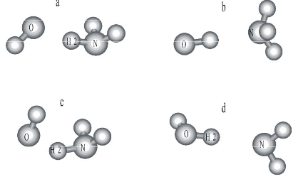
Figure 6.25 Bond rearrangements that occur during the OH- (NH3) OH2 NH2- reaction [253].
In Fig. 6.26, we see the gas-phase reaction energy profile that the Lineberger group was able to infer based upon their anion spectroscopic study combined with ab initio calculations they carried out.
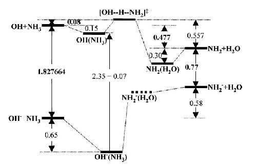
Figure 6.26. OH···NH3→ TS → OH2···NH2 energy profile inferred from anion spectroscopic measurements.
Again, because OH + NH3→ OH2 + NH2 is exothermic as shown in Fig. 6.26, the transition state of this reaction will be closer in structure to OH···NH3 than to OH2···NH2. Therefore, to probe this transition state, it would be best to use the OH-···NH3 complex as a precursor.
Let us now return now to the first point made when we discussed the OH-(H2) case, which was that both H-(H2O) and (OH-)(H2) are stable local minima on the same ground-state energy surface. Hence, one must take care to prepare samples that contain (primarily) the isomer one wishes to study. In addition to the above two isomers, the double-Rydberg anion (H3O)- also lies on this same energy surface (we discussed double-Rydberg anions in greater detail in Chapter 4). This species consists of a hydronium cation (H3O+) with a pair of electrons attached to its lowest-energy a1-symmetry Rydberg orbital as shown in Fig. 6.27 [[254]] from Professor Vince Ortiz's group. The double-Rydberg anion binds its excess electron by only ca. 0.5 eV.
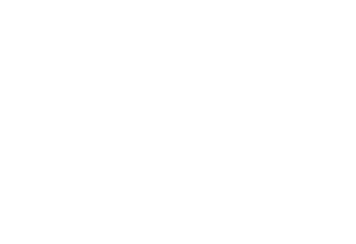
Figure 6.27. Lowest-energy Rydberg orbital of H3O+ which contains two electrons in the double-Rydberg (H3O)- anion.
So, one must be fully aware of which isomer exists in an experimental source if one hopes to properly interpret photoelectron spectra or other data on that sample. Of course, by selecting proper precursors (e.g., OH- if one wishes to form OH-(H2)) and controlling experimental conditions (e.g., keeping the internal energy low to avoid isomerization), one can usually minimize such difficulties. However, there are times when even such efforts do not suffice.
Another example [[255]] from Professor Piotr Skurski's lab of a cluster anion with more than one kind of geometrically stable structure is provided by the (NaCl)2- cluster. As shown in Fig. 6.28, this anion has a quasi-linear dipole-bound anion structure (1- and 2-), a rhombic quadrupole-bound anion structure (3-), and a solvated-electron structure (4-). So, it is possible for a cluster of one stoichiometry to display a variety of electron-binding motifs.
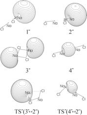
Figure 6.28 The (NaCl)2- dimer anion has four stable isomers (1- to 4-) and transition states (TS) that connect them.
Next, I want to discuss a class of experiments that is similar to what we outlined earlier for using electron photodetachment to probe reactions on the corresponding neutral-molecule potential energy surface but which yield other important dynamical information. The research group of Professor Carl Lineberger has used the fact that some molecular anions have geometrically bound ground states but dissociative electronic excited states to probe the dynamics of the recombination process. For example, the I2- anion, whose solvation structure with CO2 solvent molecules was discussed earlier in this text, has an excited state I2-* that dissociates to I + I- (in fact, there are two spin-orbit split states that produce I(2P3/2) and I(2P1/2), respectively). This excited state can, alternatively, undergo radiationless relaxation and return to the ground state of I2-, but if it does return to the ground state, it produces I2 with a great deal of vibrational energy (we denote this vibrationally hot speciesI2-(vib)). The Lineberger group has learned a great deal about energy deposition/transfer and solvation structure in a series of experiments in which the following photoinduced reactions are studied:
I2-(Sol)N + hn → I2-(Sol)N*
I2-* (Sol)N→ I(Sol)N-K + I-(Sol)K-L + L (Sol).
I2-*(Sol)N-M + M (Sol) ← I2-(vib)(Sol)N← I2-* (Sol)N
That is, the mass-selected solvated anion cluster is excited (the first reaction above), after which some of these anions fragment to yield I- anion and I neutral in various solvation states as well as some solvent species (the second reaction). Alternatively, some of the excited solvated anions relax to the ground electronic state and subsequently boil off some of their solvent molecules producing a less-solvated ground-state anion (the third reaction). By using mass-specific detection to examine the relative abundances of the various products in such experiments, the Lineberger group has generated a wealth of new insight into the solvation of anions and into intra-molecular energy-transfer rates and mechanisms.
IV. Sometimes the Isomers are New Anions
There is an interesting story behind what lead to the discovery of so-called double-Rydberg anions in Professor Kit Bowen's laboratory in 1987 [[256]]. These workers were examining the photoelectron spectrum of solvated hydride ions. Specifically, in one experiment, they were studying the photoelectron spectrum of H-(H3N), which is shown in Fig. 6.29.
Figure 6.29. Photoelectron spectrum of H- (top) and of H-(NH3) (middle) [256].
The spectrum of H-(NH3) clearly shows a large peak whose electron binding energy (ca. 1.2 eV) exceeds that of H- (0.75 eV), as expected because the solvation energy of H- exceeds that of neutral H. However, when the data in the neighborhood of this primary peak was examined in further detail as shown in Fig. 6.30, another (minor) peak was discovered.
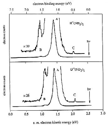
Figure 6.30. Primary peak (A) and minor peak (C) in photodetachment spectrum of H-(NH3) [256].
The minor peak C is seen to have an electron binding energy of ca. 0.4 eV, which is less than that of H-. The puzzle that faced researchers at that time was to suggest what species with the stoichiometry of NH4- would explain peak C. Of course, the possibility that the peak may belong to NH2-(H2) was considered, but this was determined to not be the source of peak C. As Professor Vince Ortiz showed, the answer [[257]] turned out to be the so-called double-Rydberg isomer of NH4-, which is shown in Fig. 6.31.
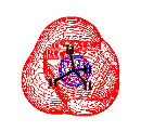
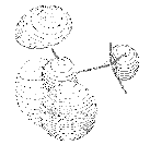
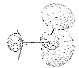
Figure 6.31. NH4- anion with its Rydberg orbital surrounding the molecular core (left); Rydberg orbitals of protonated methyl amine (center) and protonated methyl alcohol (right).
The NH4- anion can be viewed as a closed-shell NH4+ cation surrounded by its lowest-energy Rydberg orbital in which a pair of electrons resides. Likewise, H3C-NH3- is protonated methyl amine with two electrons occupying its lowest Rydberg orbital [254].
V. Covalent and Metallic Cluster Anions
In addition to the solvated-anion and solvated-electron type clusters discussed earlier in this Chapter, at least two other families of cluster anions are commonly encountered. These include:
- clusters of atoms covalently bonded to one another with an excess electron attached, as well as
- clusters of metallic atoms with an excess electron attached.
We differentiate between these two families because the basic nature of their electronic bonding is qualitatively different. In the former, one has a network of atoms linked together by directed covalent bonds such as is shown in Fig. 6.32 for two silicon clusters
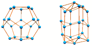
Figure 6.32. Clusters of Si atoms showing their network of directed bonds.
Notice that the some of the Si atoms in these clusters are bonded to four other Si atoms as one expects for a tetra-valent aton, whereas some are linked to only three others (especially in the smaller cluster on the left). The latter have what are called dangling bonds; that is, they possess one unused sp3-type orbital (each containing a single electron). The presence of these dangling bonds renders these atoms highly reactive radical-like centers. In both clusters shown in Fig. 6.32, we see not only four- or three-fold coordination but also (approximately, because these structures contain substantial strain) the expected bond angles that accompany sp3 hybridization. The fact that each Si atom's valence electrons can be accounted for in terms of sp3 orbitals each containing one electron underlies why we view these clusters as covalently bonded.
Silicon surfaces also contain atoms that are bonded to only three others and thus have such dangling bonds. Of course, on a silicon surface, the layers of atoms can buckle (this is called reconstruction) and allow surface Si atoms to approach one another closely enough to form bonds. The study of the behavior of such surface dangling bonds plays a central role in surface science because of the high reactivity of such sites. Because small clusters usually contain a higher fraction of under-coordinated atoms, they are often viewed as excellent test beds for studying the behavior of atoms on surfaces and as prototypes of reactive surfaces.
Other examples of covalently bonded cluster anions are illustrated in Professor Will Castleman's group's study [[258]] of gold-oxygen cluster Au(O)n- anions several of whose structures are shown in Fig. 6.33 and of Al(N)n- cluster anions [[259]] depicted in Fig. 6.34.
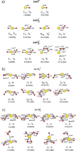
Figure 6.33. Structures of several Au(O)n- cluster anions also showing their point group and spin symmetries and energies (kcal mol-1 in parantheses) relative to the lowest-energy isomer for each species.
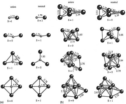 Figure 6.34 Structures of several Al(N)n- cluster anions also showing their spin symmetries.
Again, we see in all of these clusters strongly spatially directed bonding that derives from the chemical valences of the atoms involved.
An especially interesting and widely studied class of clusters derives from work in Professor Will Castleman's lab on so-called Met-Car clusters [[260]] consisting of a cluster of early transition metal atoms combined with carbon atoms. Originally, a Met-Car such as Ti8C12 was thought to consist of a cube of eight Ti atoms (each contributing four electrons 4s2 3d2) and one C2 unit sitting on each of the six faces of the cube. However, it was subsequently determined that Ti8C12 has the structure shown in Fig. 6.35.
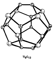 >
>
Figure 6.35. Dodechahedral structure of Ti8C12 [[261]].
In a photoelectron spectroscopy study of the Ti8C12- anion [[262]], Professor Lai-Sheng Wang's group determined that the electronic structure of this species can be viewed as follows:
- The eight Ti atoms each contribute four electrons;
- Of these thirty-two electrons, twelve can be viewed (i.e., counted) as being donated to the six C2units to form the closed-shell C22-ions (n.b., these dianions are certainly not stable as isolated species, but they can be stabilized by the Ti counter ions);
- The remaining twenty electrons occupy the molecular orbitals as shown in Fig. 6.36.
In this figure, all of the orbitals have dominant Ti-atom character; the C22- units are treated as closed-shell ions that serve only to symmetry-split the Ti-derived orbitals.
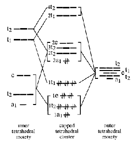
Figure 6.36. Molecular orbitals in Ti8C12 (center) constructed from the Ti orbitals.
The fact that the last two electrons occupy the high-energy 2a1 orbital is consistent with the low ionization potential (4.9 eV) of the neutral Ti8C12. The presence of the 2t2 orbital somewhat above this 2a1 orbital suggests that Ti8C12 should have a rather low EA, and it does (ca. 1.1 eV). Finally, the orbital diagram shown in Fig. 6.36 suggests that the Ti8C122+ dication should be especially stable because it has a closed-shell and because its HOMO-LUMO energy gap (i.e., the 1t1-2a1 gap) is large.
The multitude of geometries that occur in the kind of clusters discussed in this Section of this Chapter presents one of the most severe challenges to their theoretical study, especially if one is faced with the task of determining which geometry has the lowest energy or which structures are prevalent in a given experiment (where free energy and the means of preparation play key roles). The difficulties derive primarily from the fact that the number of atoms in even a modest size cluster can be connected together in many different ways subject only to the constraints dictated by the valence of the constituent atoms. One has to consider all such connections to address the issue of what structure is the global minimum on the energy surface and to characterize those structures that have experimentally accessible energies. Because the number of such structures grows exponentially with the number of atoms in the cluster, this task becomes overwhelming even for modest numbers of atoms. In addition, especially when clusters have unpaired electrons, one must consider various spin states in searching for the low-energy structures for a cluster of a given stoichiometry.
In contrast, for metallic clusters, the situation is usually simplified by the fact that the outermost valence electrons of the atoms (e.g., s1 for Cu, Ag, or Au; s2 for Ni or Mg) are delocalized over the entire cluster rather than localized within valence-directed orbitals. That is, because metals have low ionization potentials, their valence orbitals tend to form delocalized bands of orbitals among which these valence electrons are distributed.
There exists a useful picture of maximal delocalization of the valence electrons that forms the basis of the so-called jellium model for the electronic structure of metallic clusters. In this model, each of the N atoms A in the cluster is assumed to donate its n valence electrons to the delocalized bands of electrons and to thus become an A+n cation. The Nxn electrons occupying the lowest-energy orbitals in the bands will have the lowest total energy when the volume of the cluster is as large as possible. The maximum volume produces the lowest energy because the model assumes a particle-in-a-box type expression (E = n2h2/8mL2) for the energy levels. This energy-minimization criterion suggests that the N cations be packed into a spherical (or nearly so) shape to form the cluster. Within this volume, the N A+n cation centers are assumed to be distributed as uniformly as possible (again to minimize the energy), and the Nxn electrons are allowed to fill the band orbitals appropriate to such a spherical volume.
So, the jellium model says the highly delocalized nature of metal clusters' valence electrons and the rather isotropic (i.e., nearly spherical) arrangements of the metal-atom core ions within the clusters allow one to describe the orbital energies of the cluster orbitals in terms of the orbitals of a particle in a spherical box of radius R0. The size of the box is, in turn, determined by how many N atoms form the cluster and the radius rA of each such atom's valence orbitals. Specifically, the total volume of N atoms A (4/3 N p rA3) is equated to the volume of the spherical cluster (4/3 p R03) to obtain an expression for R0 in terms of the atomic radius rA and the number of atoms in the cluster N
R03 = N rA3.
For such a box of radius R0, an electron in an orbital having angular momentum L will have an energy Ek, L determined from the condition that the Lth spherical Bessel function JL vanish at the boundary of the box:
JL((2meE/h2)1/2R0) = 0.
Of course, for each L, there are many values of E for which the JL function vanishes, so there are, as expected, many energy levels for each L value. The values of x ≡ ((2meE/h2)1/2R0 that cause the Lth Bessel function to vanish are displayed in Fig. 6.35 for L = 0, 1, and 2 (i.e., for S, P, and D spherical-box orbitals). The energies Ek,L appropriate to each L value are obtained by squaring the numerical values of x shown in Fig. 6.37 and using E = (h2x2)/(2meR02). As a result, the spacings between orbitals of a given L grow as one moves up the energy ladder for that L.
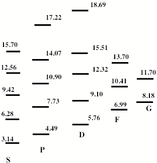
Figure 6.37. Energy levels of the particle in a spherical box jellium model for L values of 0, 1, 2, 3, and 4, showing the x values of each level.
Notice that closed-shell electronic structures are predicted to occur when 2, 8, 18, 20, 34, 40, etc. valence electrons occupy the band orbitals. There are also less stable, yet noticeably favored, half-filled shell states when 5, 13, 19, 27, etc. electrons are present. These magic numbers are indeed observed in metal-atom clusters as such clusters seem to display special stability to electron gain or loss as well as inertness to chemical reaction (especially for the closed-shell structures that possess no half-filled radical-like orbitals). An example from Professor Carl Lineberger' lab [[263]] of such magic number stability is shown in Fig. 6.38 where the electron detachment energies of copper. silver, and gold clusters are plotted as a function of cluster size (n).
Figure 6.38. Electron affinities of copper, silver, and gold clusters vs. number of atoms (n).
Here, we see drops in EAs at cluster sizes of 2 and 8, in particular. In Fig. 6.39, also from ref. 263, the special character of clusters with 2 and 8 electrons also is clear; this figure plots the energy gap between the highest occupied and lowest unoccupied molecular orbitals in the cluster. For n = 2 and n = 8, one has closed-shell structures, so the energy gap is large here.
Figure 6.39. HOMO-LUMO energy gap in copper and silver clusters.
In contrast to the kind of metallic behavior observed in the clusters just discussed, when the EAs of clusters that involve covalently bonded atoms are measured, one does not observe such magic-number patterns. For example, the EAs of (GaAs)n clusters as a function of cluster size n are shown in Fig. 6.40.
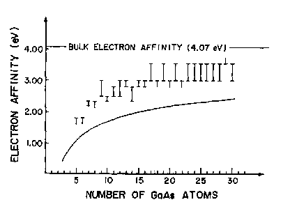
Figure 6.40. Electron affinities of (GaAs)n clusters vs. cluster size n.
For clusters of such main-group atoms that are not all that metallic, a smoother trend of EA vs. cluster size is observed. In particular, for the (GaAs)n clusters, the measured EAs approach the EA of bulk GaAs(s) (i.e. the work function) of 4.07 eV as the cluster size grows.
Another example from Professor Kit Bowen's lab [[264]] involves the evolution of Mgn clusters toward metallic behavior as the cluster size increases. Recall that Mg has two electrons in its 3s valence orbital, but the 3s-to-3p promotion energy is small. As one constructs Mgn clusters (conceptually) by adding more and more Mg atoms, one expects to see an evolution in the bands comprised (largely) of 3s and 3p orbital character much as we see in Fig. 6.41 from ref. 264.

Figure 6.41. Qualitative orbital energy diagram for Mg 3s and 3p orbitals evolving from bonding, non-bonding, antibonding molecular orbitals (toward the left) into bands of orbitals (right).
This depiction suggests that there will be a gap (denoted by the D symbol in Fig. 6.41) between the 3s- based and 3p-based bands for intermediate cluster size prior to the bands overlapping as Mg becomes a metal.
Because each Mg atom has two valence electrons and both 3s and 3p orbitals, the counting involved in defining magic numbers is a bit more complicated than we discussed above for the jellium model where each atom was assumed to contribute one electron and one orbital. Nevertheless, we see in the mass spectrum of Mg shown in Fig. 6.42 that certain Mgn- cluster anion sizes (e.g., 4, 9, 19, 34, etc. having 8, 18, 38, and 68 electrons, respectively) seem to be especially abundant. This, in turn is taken to mean these magic clusters possess special stability, probably related to a closed electronic shell structure.
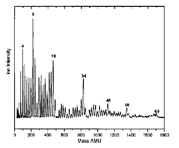
Figure 6.42. Abundances of Mgn- ions observed in mass spectrum of magnesium showing the existence of magic cluster sizes.
By also carrying out photoelectron spectroscopy on mass-selected Mgn- anions and looking both at the energy needed to remove an electron (nominally one of the 3s electrons) as well as the energy needed to remove a 3s electron and excite a second electron from 3s to 3p, the Bowen group was able to determine the 3s-to-3p energy gap for clusters of various sizes. A plot of these energy gaps for various cluster sizes appears in Fig. 6.43.
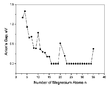
Figure 6.43. Mgn- 3s-3p energy gap as a function of cluster size.
Considering the qualitative orbital pattern displayed in Fig. 6.41, one expects to see the 3s-3p energy gap vanish when the 3s and 3p bands overlap and Mg thus becomes metallic. Based on the data of Fig. 6.43, the Bowen group concluded that Mgn clusters larger than ca. 18-20 should be metallic.
Let's consider a cluster in which both metal and non-metal atoms occur. For many years, chemists have been interested in making a compound in which carbon has a square planar bonding arrangement. In 1998, Professor Alex Boldyrev and the author [[265]] suggested a bonding paradigm within which this might be possible. We suggested that a carbon atom could use its 2s and two in-plane (x,y) 2p orbitals to form one 4-center and a pair of 3-center bonding orbitals to ligands as depicted qualitatively in Fig. 6.44.

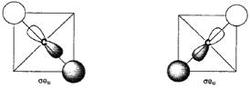
Figure 6.44. 4-center and 3-center carbon-ligand bonding orbitals in square planar geometry.
If the ligands also possess out-of-plane p-type valence orbitals, the central carbon atom can use its remaining 2p (z) orbital to form a 5-center p-type bonding orbital as shown in Fig. 6.45. Finally, the ligands can use their in-plane p-type orbitals to form a 4-center ligand-ligand bonding orbital also shown in Fig. 6.45.
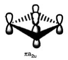
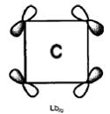
Figure 6.45. p-type 5-center and in-plane 4-center ligand-ligand bonding orbitals.
Then, using four valence electrons from the carbon atom and a total of six more electrons from the ligands, one can form three in-plane carbon-ligand bonds, one out-of-plane carbon-ligand bond, and one in-plane ligand-ligand bond. In this way, we suggested, for example, that species such as CSi2Al2, CSi2Ga2, and CGe2Al2 might be stable. In these compounds, the Si and Ge atoms each contribute two electrons (their p electrons) and the Al and Ga atoms contribute one electron (their p) to the bonding; these atoms s2 electrons are not involved in forming the bonds.
Notice that alkaline earth atoms would not be optimal to use as ligands because one would have to promote them from s2 to s1p1 character so they could use their p orbitals to form some of the bonds discussed above. Also note that the sizes of the atoms used as ligands is important; for example, Sn and Pb might not be good substitutues for Si because the C-Sn or C-Pb orbital overlaps would be less favorable than for C-Si. That is, the atoms have to be of the right sizes to fit together to form a feasible structure.
After putting forth the above bonding paradigm, we then went on [[266]] to examine the CAl4- cluster anion (n.b., this involves nine electrons so it has only one electron in the 4-center ligand-ligand bonding orbital in the bonding scheme just discussed). We found the highest-occupied molecular orbitals of this cluster to have the character shown in Fig. 6.46.
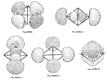
Figure 6.46. The five highest-energy molecular orbitals of CAl4-
The HOMO is the 4-center ligand-ligand in-plane bonding orbital that contains one electron in CAl4-. The HOMO-3 orbital is the 5-center p-type carbon-ligand bonding orbital, and HOMO-1, HOMO-2, and HOMO-3 are non-bonding (e.g., Al 3s) orbitals localized mainly on the Al ligands. The three other in-plane bonding carbon-ligand orbitals lie below HOMO-3. The photoelectron spectum observed for this CAl4- ion indeed matched well what our theoretical ion-neutral energy difference predicted for the square planar structure. In particular, a broad Franck-Condon envelope was observed in the transition leading from (square planar) CAl4- to the ground electronic state of neutral (tetrahedral) CAl4. In addition, the theoretically calculated energies of various excited states of neutral CAl4 agreed well with other peaks seen in the photoelectron spectrum.
The team of Professors Alex Boldyrev and Lai-Sheng Wang have studied a huge number of other novel cluster anions, many of which they summarize in a review article [[267]]. One of the building block anions that they use (along with isoelectronic analogs) is the Al42- dianion which forms a tetrahedral structure. The higher-energy occupied molecular orbitals of this species are shown in Fig. 6.47.
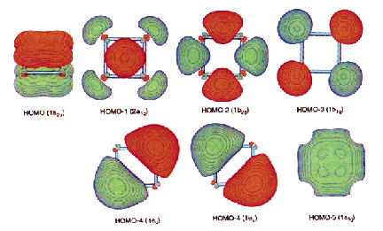 Figure 6.47. Higher-energy occupied orbitals of Al4-.
The HOMO is an out-of-plane p-bonding orbital involving all four Al atoms. HOMO-1 is an in-plane bonding orbital involving all four Al atoms, and HOMO-2 is also an in-plane bonding orbital but it involves tangential bonding between neighboring Al atoms around the periphery. The six electrons that occupy these three orbitals form the bonding framework that holds Al42- together. HOMO-3 through HOMO-5 are comprised mainly of Al 3s orbitals; the eight electrons occupying these four orbitals have no significant net bonding contribution.
Chapter 7. Anions of Biological Molecules
The anions formed by attaching an electron to a biological molecule are not qualitatively different than those that have already been discussed. They include dipole-bound and valence-bound anions, solvated anions, zwitterion anions, metastable anions, and cluster anions. However, because of the great importance of molecules that arise in living organisms and because bio-molecules often possess a variety of structural and geometrical isomers to consider, much attention has been devoted to such species, especially in recent years, so I felt it appropriate to consider the effects of attaching electrons to such molecules in a distinct Chapter.
The research groups of Professors Ludwik Adamowicz and Kit Bowen as well as the Schaefer, Schermann-Desfrançois, Burrow, Märk, and Illenberger groups have been involved in many experimental and theoretical studies of anions involving biological molecules. These investigations have focused on dipole-bound anions, valence-bound anions, and anions arising from binding an electron to a cluster containing one or more biological molecule. Most, if not all, of the experimental studies from the groups just mentioned have involved gas-phase samples of individual bio-molecules or pairs of such molecules, and, in some cases, with one or a few water molecules attached. Most of the theoretical studies have also focused on these types of systems. Professor Léon Sanche and Professor Ron Naaman have studied electrons attaching to bio-molecules that exist in condensed media including such as dried DNA samples and self-assembled mono-layers of single- and double-strand DNA oligomers. In this Chapter, we will be discussing each of these situations in which electrons bind to biological molecules.
I. Dipole-bound and Valence Anions
As the first example of such bio-molecules from a collaboration [[268]] of the Schermann-Desfrançois team and Professor Ludwik Adamowicz, in Fig. 7.1 we show the structure of the indole-water anion complex as well as the orbital occupied by the excess electron in this case. I chose to begin with this species because I think most readers would expect such an anion to consist of an indole ion holding an electron in a valence p* orbital with the water molecule solvating this anion. However, such is not the case.
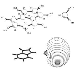
Figure 7.1. Structure (top) of indole-water anion complex and orbital (bottom) occupied by excess electron.
Clearly, this is an example of a dipole-bound anion in which the dipole potential is formed by combining the dipoles of the indole and the attached water molecule. I remind the reader that an individual H2O molecule does not have a large enough dipole moment to bind an electron. So, even though the dipole-bound orbital may appear to be located on or near the positive side of the water moiety, its existence derives not from the dipole potential of the water molecule alone but from the combined dipole potential of the indole-water complex. It is also useful to note that this anion cannot correspond to an indole anion that has been solvated by the one water molecule shown. If that were the case, the water molecule would have its H atoms directed toward rather than away from the indole and the orbital holding the excess electron would be localized on the indole or between the indole and the water molecule.
As another example of a bio-molecule anion derived from Professor Fritz Schaefer's work [[269]], we show in Fig. 7.2 the structure of a valence-bound anion that results from attaching an electron to a p* orbital of an adenine-thymine hydrogen-bonded base-pair complex as occurs in DNA. Because thymine's lowest-energy p* orbital lies below that of adenine, it makes sense that the lowest p* orbital of the complex would be primarily localized on the thymine as shown, although it clearly shows a small degree of delocalization onto the adenine. This indicates that the p-orbitals of A and of T are indeed coupled even though there is a spacer unit consisting of the in-plane hydrogen bonds connecting A to T.
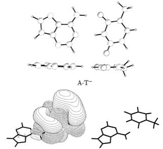
Figure 7.2. Geometry of adenine (left)-thymine (right) anion complex (top) and valence p* orbital containing the excess electron (bottom left).
Additional insight from Professor Fritz Schaefer's group into this situation is offered in Fig. 7.3 where the singly occupied molecular orbitals (SOMO) of adenine, thymine, and of the A-T complex are displayed, again illustrating that the SOMO of A-T- is more similar to that of T- than to that of A-.
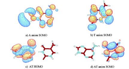
Fig. 7.3. Singly occupied molecular orbitals of adenine anion (a), thymine anion (b) and of the AT complex anion (d).
Not surprisingly, one also finds that, for the guanine-cytosine complex [[270]], the anion's SOMO is similar to that of cytosine because the cytosine anion binds its excess electron more tightly than does the guanine anion. The pertinent SOMOs are shown in Fig. 7.4.
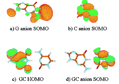
Figure 7.4. Singly occupied molecular orbitals of guanine anion (a), cytosine anion (b) and of G-C complex anion (d).
It is also useful to point out that when an excess electron attaches to such a base pair and is more highly localized on one of the bases, it causes a larger geometrical deformation on that base. For example, in Fig. 7.5 we show the equilibrium geometries found in ref. 270 the neutral GC base pair and of the GC- anion where it is clear that the geometry of the cytosine moiety is more deformed by the addition of the electron than is that of the guanine.
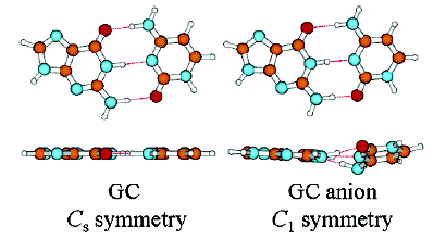
Figure 7.5. Equilibrium geometries of guanine-cytosine base pair (left) and of the corresponding anion (right).
This knowledge about how an excess electron is more localized on the cytosine and thymine bases should be kept in mind if one is studying how electrons migrate up and down p-stacked chains of bases in double strands of DNA.
In Fig. 7.6 we see an illustration of a case studied in the author's group [[271]] in which an electron can attach to more than one site. In this example, a model of a disulfide linked species +H3N-(CH2)3-S-S-CH3 with a nearby protonated amine site (both of these groupings occur in peptides and proteins) is used to show that the electron can attach to the protonated site to form a Rydberg-attached species or to the S-S anti-bonding s* orbital to cleave the S-S bond.
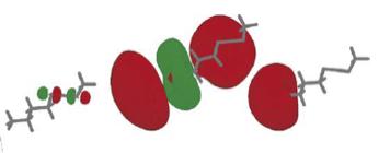
Figure 7.6. Electron attached to S-S s* orbital (left), to +H3N- excited Rydberg orbital (center) or to +H3N- ground Rydberg orbital (right) in +H3N-(CH2)3-S-S-CH3.
Later in this Chapter I will have more to say about the importance of such electron attachment events. Suffice it to say for now that peptide mass spectrometric fragmentation patterns suggest that the kind of Rydberg- and anti-bonding orbital- attachment processes involving the above orbital occupancies play central roles in electron-induced fragmentations of peptides and proteins.
One also should be aware of the fact that when electrons attach to one orbital, they do not always remain there. One thing that can happen is that they can migrate (undergoing so-called through-bond or through-space electron transfer) onto another orbital. An example from the author's group [[272]] of this is given in Fig. 7.7 where we show an electron initially attached to a cytosine p* orbital (in a cytosine-sugar-phosphate DNA fragment) that subsequently migrates onto a sugar-phosphate C-O s* orbital. In this case, once the electron enters the s* orbital, the sugar-phoaphate C-O bond cleaves and a so-called single strand break is formed.
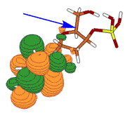
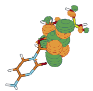
Figure 7.7. Electron attached to cytosine p* orbital (left) that migrates through the sugar moiety onto the sugar-phosphate C-O bond's (blue arrow) s* orbital (right).
The above examples serve to illustrate that an electron can attach to valence or to dipole orbitals of bio-molecules. Later in this Chapter, I will discuss in considerable detail what can happen when an electron attaches to DNA or to a peptide or protein. However, before undertaking those subjects, it is important to first deal with the fact that some of the anionic states encountered in bio-molecules are electronically metastable.
II. Virtual Orbitals May Not be Electronically Stable
It is informative to mention at this time how the energies of the p* orbitals appearing in some of the examples discussed earlier in this text are determined experimentally using a so-called electron transmission spectrum (ETS). Professors Paul Burrow's and Michael Allan's groups have made many pioneering advances in the development and application of this novel spectroscopic tool. One might think that electronic absorption spectroscopy, in which an electron is excited from a lower-energy orbital into a p* orbital, could provide this information. However, this is not the case. When an electron is excited from an occupied orbital to a p* orbital, this electron feels an attractive Coulomb potential at large r because it is an orbital of a neutral molecule, not of an anion. That is, the excitation process leaves a hole behind and this hole has a net positive charge that binds the p* electron. In contrast, an excess electron entering a neutral molecule's p* orbital (to form an anion) does not feel any such long-range Coulomb potential; instead it experiences only shorter-range dipole or other potentials. The bottom line is that the p* orbital of the anion is not the same as the p* orbital formed by electronically exciting the molecule; the former is significantly more diffuse than the latter and it has to be characterized using special tools such as ETS spectroscopy.
In an ETS kind of experiment, a beam of electrons having well defined kinetic energy E is allowed to impinge on a sample (e.g., a gaseous sample containing adenine-thymine complexes). The intensity I0 of the incident electron beam is measured as is the intensity I of the beam that is transmitted through the sample. As the kinetic energy of the incident electrons is varied, eventually the kinetic energy reaches a value that corresponds to the energy of one of the unoccupied orbitals of the neutral molecule. It is at such energies that electron attachment can most likely occur, and the transmitted electron beam will be attenuated by these capture events.
A Beer-Lambert type expression is then used to determine the extinction coefficient e[E] appropriate to electrons of energy E:
log (I0/I) = e C L.
Here, C is the concentration of molecules that can attach an electron of energy E and L is the path length of the sample through which the electron beam traverses. It turns out that most ETS spectrometers determine not e[E] but the derivative de/dE of the signal with respect to the electron energy E. So in the ETS spectra from Professor Paul Burrow's group [[273]] shown in Fig. 7.8 for thymine, cytosine, guanine, and adenine (as well as uracil) it is not where the peaks occur that determine the electron attachment maxima but the inflection points where the vertical lines are shown. Where e[E] has a minimum (no absorption) or a maximum (a peak), de[E]/dE vanishes. However, de[E]/dE has minima at inflection points on the e[E] curve lying between a minimum and a peak but below the peak energy. On the other hand, de[E]/dE has maxima at inflection points on the e[E] curve lying between a peak and a minimum but above the peak energy. Hence, between minima and maxima in the de[E]/dE plots lie the peaks in e[E].
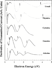
Figure 7.8. ETS spectra of DNA bases and of uracil with the vertical lines marking peaks in e[E].
From this data, one sees that thymine's lowest p* orbital (at ca. 0.3 eV) lies below that of adenine (ca. 0.5 eV); likewise cytosine's lowest p* orbital lies below guanine's. The features shown in an ETS spectrum have significant width in large part because the anion states formed upon electron attachment have very short (usually < 10-14 s) lifetimes so they have large Heisenberg widths (a lifetime of 10-14 s corresponds to a width of ca. 0.4 eV).
There are variants of ETS spectroscopy in which one measures not the attenuation of the incident electron beam but the intensity of electrons deflected at right angles to the incident beam. These strongly scattered electrons have major contributions from processes in which an electron is captured and retained by the molecule long enough for substantial rotational or vibrational motion to occur. By measuring the kinetic energies of these scattered electrons, one can gain information about the vibrational energy spacings within the metastable molecular anion. An example from Professor Michael Allan's lab [[274]] is shown in Fig. 7.9 where we see an energy-loss spectrum for the formic acid molecule HCOOH.
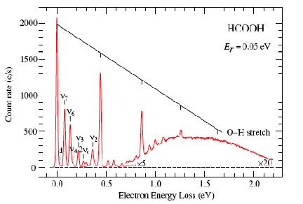
Figure 7.9. Electron energy-loss spectrum for formic acid HCOOH.
In this spectrum, there are several distinct peaks that have been labeled by their vibrational mode number n1 (the OH stretch) through n7 (OCO deformation). These data suggest that the OH stretching mode, in particular, can be excited to at least its v = 4 level by electron impact at energies near that of the C=O p* resonance state of the corresponding anion.
Because these electron-attached states are metastable with respect to auto-detachment, their theoretical treatment is also complicated. Specifically, one cannot use conventional electronic structure theory to study them. One must either approach their study using electron-molecule scattering theory as, for example, Professor Chris Greene has done [[275]] for DNA fragments or one must employ one of the stabililization techniques discussed in Chapter 5.
From the examples discussed thus far, we see that bio-molecules and their hydration complexes can form dipole-bound, Rydberg-bound, and p* valence-bound anions. Which of these anions lies lower in energy and which will be formed in a particular experimental situation depends upon how the anion is formed. Specifically, it depends on the geometry of the underlying molecular framework. To illustrate this point, in Fig. 7.10 from the Schermann-Desfrançois group we show the energy landscapes of a uracil molecule [[276]] and of its dipole-bound and p* valence-bound anions as functions of a coordinate describing the ring puckering deformation that occurs when an electron is attached to form the p* anion. Both the neutral and dipole-bound anion have equilibrium geometries that are not (significantly) deformed along this coordinate, whereas the equilibrium geometry of the valence-bound anion is substantially puckered.
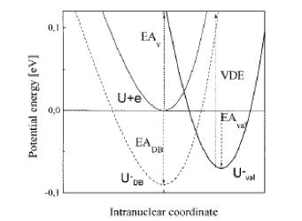
Figure 7.10. Schematic depiction of the energy of neutral uracil (U) with an electron far from it (U+e) as a function of ring deformation coordinate as well as the energies of the dipole-bound uracil anion (U-DB) and the p* valence-bound uracil anion (U-val) along this same coordinate.
Clearly, if an electron strikes a neutral uracil molecule (e.g., as in an ETS experiment), it will encounter the uracil having a configuration near its planar equilibrium geometry. At such geometries, the p* valence-bound anion lies more than 0.1 eV above the neutral, and thus is a metastable resonance state (and one should use a stabilization-type theory to describe it as discussed in Chapter 5). At these same geometries, the dipole-bound anion lies below the neutral and is a bound state, but can not be formed by direct electron attachment unless a third body is present to carry away the ca. 0.1 eV of exothermicity or if vibrational excitation accompanied the attachment process (the latter process is called a vibrational Feshbach event). The dipole-bound state could, however, be formed efficiently if the neutral U were to collide with, for example, a Rydberg excited atom (e.g., Cs**) whose IP (i.e., energy to effect Cs** Cs+ + e-) were resonant with the EA of U to form the dipole-bound state. This is, of course, the route that the Schermann-Desfrançois group uses to form such dipole-bound states of bio-molecules.
In contrast, if the uracil's ring were sufficiently distorted, an electron can attach and form an electronically stable p* valence-bound anion that lies adiabatically 0.07 eV and vertically more than 0.2 eV below the neutral U. Such valence-bound anions can also be formed by colliding neutral uracil with a highly excited Rydberg state of a Cs atom Cs**. If the energy needed to ionize the Cs** (to form Cs+) matches the energy gained in moving adiabatically from U to U-val, an electron can efficiently be transferred from the Cs to the uracil. Such resonant electron transfer processes can be used to induce adiabatic changes because they occur slowly on the electronic time scale (because they involve a slow molecuular collision between Cs** and U).
An example of a vibrational Feshbach resonance being involved in forming a dipole-bound anion is offered by work from Professors Paul Burrow's and Tilmann Märk's groups [[277]] involving uracil. In Fig. 7.11 we see three potential energy curves and a depiction of the N-H s* orbital of uracil.
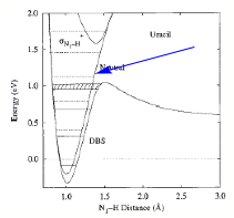
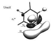
Figure 7.11. N-H s* orbital of uracil (right) and energies of neutral, dipole-attached, and N-H s*-attached uracil anion (left) as functions of the N-H bond length.
The workers of ref. 277 suggest that an electron can, for example, attach to a neutral uracil molecule having its N-H stretching vibration in the v = 0, 1, or 2 level to produce the dipole-bound uracil anion in the v = 1, 2, or 3 level. The exothermicity arising from the attachment to form the dipole state, combined with the electron's kinetic energy, allows the vibrational excitation to occur. The vibrationally excited dipole-bound state then couples with the N-H s*-attached state as the N-H bond elongates to produce a barrier (arrow) on the anion surface. Accessing and crossing this barrier then determines the rate at which the N-H bond is cleaved in this dissociative electron attachment (DEA) event.
III. Electrons Attached to DNA
As mentioned earlier in Chapter 4, the relevance of DNA's bases' and other biomolecules' dipole-bound anions in living organisms can be questioned because it is highly unlikely that in vivo the regions of these bases' attractive dipole potentials are exposed and accessible to an electron that may approach. Instead, the region of space where the dipole potential is strongest probably is occupied by a solvent molecule or some other nearby species.
However, the importance of the p* valence anion states of such species is probably substantial in condensed-phase environments. In fact, it is believed that electrons migrate along strands of DNA by first attaching to a p* orbital of a base pair and then migrating to a p* orbital of a neighboring (i.e., above or below in the p-stacked helical structure) base pair as the p* orbitals on these neighborsd overlap and thus allow electron transfer. Of course, the dynamical puckering of the two base pairs involved in the electron transfer up and down the DNA chain can play an important role in gating or promoting the electron's migration because out-of-plane puckering modulates the electron binding energies of the bases as we discussed earlier in this Chapter.
Let us consider an example of a valence-bound anion of a bio-molecule, the anion arising from attaching an electron to one of DNA's four bases' p* orbitals with the base attached to a deoxyribose moiety which is, in turn, attached to two phosphate groups as in DNA itself. The author's work in this area was inspired by novel experimental findings [[278]] from Professor Léon Sanche's group in which strand breaks in DNA were produced by electrons having kinetic energies as low as 3 eV (see Fig. 7.12). The plasmid E. coli. DNA samples were suspended in nanopure water and subsequently desiccated. As a result, each such sample was very dry (containing only structural water molecules) and possessed counter cations likely near the backbone phosphate groups. Thus, the DNA samples were charge-neutral in the regions of their phosphate units. Subsequent to irradiating (at room temperature for a fixed time duration) a sample with an electron beam of known current density and known kinetic energy, the DNA sample was subjected to gel electrophoresis analysis. This analysis allowed workers of ref. 278 to quantify the amount of sample that had been undamaged, had undergone a single strand break (SSB), or had realized a double strand break (DSB) as shown in Fig. 7.12.
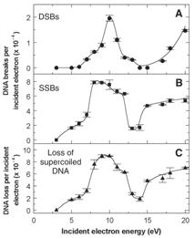
Figure 7.12. The yield of single strand breaks (middle panel) per attached electron as a function of the kinetic energy of the incident electron [278].
In other work on gas-phase samples of DNA's building blocks, it has been shown by Professors Eugen Illenberger's and Tillmann Märk's groups that the bases of DNA attach electrons to their p* orbitals and subsequently undergo cleavage of a base N-H bond as demonstrated in Fig. 1.13 [[279]]. It was also known [[280]] that, in base-sugar fragments, the base can attach an electron to its p* orbital and cleave the base-sugar N-C bond.
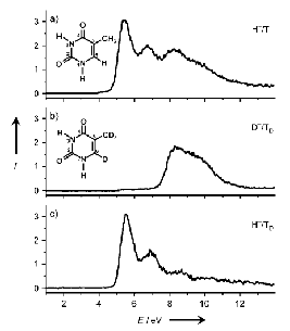
Figure 7.13. Yield of H- anions formed by dissociative electron attachment to selectively deuterated (b) thymine showing H- loss from N1 and N3 (c) positions of thymine.
The yields of single strand breaks (SSBs) in DNA were observed to depend on the kinetic energy of the incident electron in a manner (see Fig. 7.12) that suggested (because peaks and valleys appeared) some kind of resonant process. The energies at which the peaks in the SSB plots occurred did not coincide with the energies (see Fig. 7.8) of the base p* orbitals; the peaks appeared at considerably higher energies. This suggested that the SSB is initiated by electrons attaching to the DNA bases to form so-called core-excited resonance states. These states arise when an electron is captured by an electronically excited state. In the case at hand, an electron attaches to a base p* orbital and loses energy by simultaneously exciting another electron from a p to a p* orbital. This can be thought of as involving the following process: e- + p2→ p1 p*2.
In theoretical studies [[281]] by the author's group on these issues, this electron attachment was considered in detail using ab initio electronic structure methods with a focus on processes occurring at electron energies where attachment into the lowest p* orbitals of the bases [[282]] of DNA is most plausible [[283]]. In particular, this work first examined the cytosine-sugar-phosphate fragment shown in Fig. 7.14.
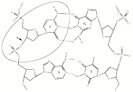
Figure 7.14. Excised portion of DNA to which an electron is attached with the C-O bond that ruptures labeled by an arrow [281].
The focus of this work was in determining how much energy was needed to break various covalent bonds in DNA because such bond cleavages produce the lesions that are called single strand breaks. After considering many different bond ruptures, we found that the phosphate-sugar O-C bond shown in Fig. 7.14 was most susceptible to cleavage when an electron is attached to the cytosine. In Fig. 7.15 are shown our plots of the electronic energies of the neutral and p* cytosine anion (both with aqueous solvation and without any solvation present) as functions of this C-O bond length.
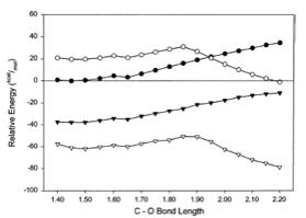
Figure 7.15 Energies of unsolvated neutral (•) and anion (○) DNA fragment and of aqueous neutral (filled ∇) and anion (∇) as functions of the sugar-phosphate C-O bond length [281].
The neutral-fragment plots show that, as expected, with or without solvation, it is energetically quite endothermic to homolytically rupture the C-O bond. Thus, it is unlikely that single strand breaks (SSBs) can occur at temperatures of 298 K, or even at significantly elevated temperature if the fragment remains neutral (i.e., does not attach an electron) whether strong solvation is present or not. The p*-attached cytosine anion energy profile is very different. It shows that, in the absence of water solvent, C-O bond rupture requires surmounting a 13 kcal mol-1 barrier and that the fragmentation process is exothermic by 21 kcal mol-1. The exothermicity results from the large electron binding energy (ca. 5 eV) of the phosphate anion -O-PO3H2 formed when the bond cleaves.
The key to understanding why the anion's C-O bond can break by surmounting a barrier of only 13 kcal mol-1 (in the absence of solvation) lies in understanding how the attached electron moves from the cytosine's p* orbital (where it is initially attached) to the phosphate's oxygen-centered 2p orbital.
In Fig. 7.16 we show three potential energy curves. One represents the energy of the neutral DNA fragment shown in Fig. 7.14 as a bond length (e.g., the sugar-phosphate C-O, a base N-H or a base-sugar N-C) is elongated. Another shows the energy of the fragment with an electron attached to the base p* orbital, while the third shows the energy of the fragment with the electron in the C-O (or N-H or N-C) s* orbital, also as functions of bond length.
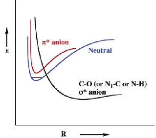
Figure 7.16. Qualitative plots of the p* (red) and s* (black) diabatic anion energy states as well as of the neutral state as functions of the C-O (or N-H or N-C) bond length R.
The two electron-attached energy curves in Fig. 7.16 cross as the bond is stretched, after which the electron can migrate, at no energy cost, from the base p* orbital onto the s* orbital. In the cytosine-sugar-phosphate example discussed above, the p* and s* curves couple near this crossing, which then allows the attached electron to migrate from the base, through the sugar, and onto the sugar-phosphate bond thus cleaving this bond. It is this avoided crossing of the p* and s* curves that produces the anion curve with a ca. 13 kcal mol-1 barrier as seen in Fig. 7.15.
In Fig. 7.17, we show the singly occupied molecular orbital (SOMO) of the cytosine anion fragment near the equilibrium value of R where the electron clearly is in the cytosine p* orbital, and at large R, where the electron resides between the phosphate and sugar groups.
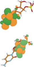
Figure 7.17. Singly occupied molecular orbital of DNA fragment for C-O bond lengths near equilibrium (top) and as C-O bond is ruptured (bottom) [281].
These plots clearly show that the attached electron migrates from the cytosine p* orbital to the phosphate, and the rate of such charge migration will be determined by the rate at which the barrier on the energy surface is surmounted as well as the rate at which the electron can move to the phosphate once the barrier is reached.
In addition to the study outlined above, this author's group also examined how an electron might attach directly to the P=O p bond of a phosphate group [[284]] and subsequently rupture a phosphate-sugar O-C bond to cause a strand break using the model compound shown in Fig. 7.18.
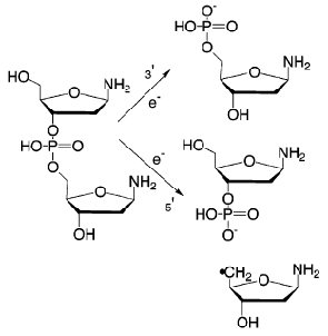
Figure 7.18. Sugar-phosphate-sugar model compound used to study C-O bond cleavage subsequent to electron attachment to phosphate P=O p* orbital.
We also looked at situations analogous to the phosphate-sugar-base model discussed above but with a thymine base in place of cytosine [[285]]. Finally, we considered [[286]] the p-stacked CCC codon shown in Fig. 7.19 with an electron attached to the central cytosine base but with two other cytosine bases above and below.
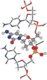
Figure 7.19. Fragment of DNA showing the three nucleotides containing cytosine–sugar–phosphate units. The C–O bond cleaved in SSB formation is marked with an arrow.
In the thymine, phosphate, and CCC electron attachment studies, the barriers to C-O bond cleavage were determined for the case where no stabilizing solvation is present when a range of solvation environments are operative. The primary finding of all these studies were the barriers to C-O bond cleavage since they determine the rates at which SSBs can occur by this mechanism, and in all cases, we determined that it is the sugar-phosphate C-O bond that has the lowest barrier to breaking. Subsequent to most of these theoretical studies, experiments from Professors Léon Sanche and Paul Burrow showed [[287]] that indeed it is primarily the sugar-phosphate C-O bonds that are cleaved when electrons enter DNA base p* orbitals.
Professor Fritz Schaefer's group [[288]] also studied the attachment of low-energy electrons to DNA fragments consisting of a base-sugar-phosphate unit. In Fig. 7.20, we see the kind of processes they studied.
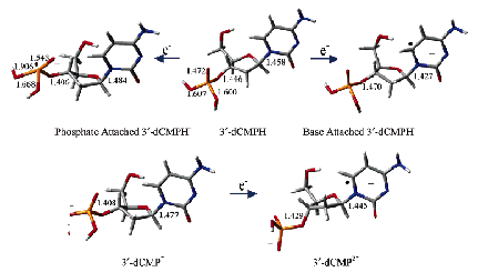
Figure 7.20. Electron attachment to phosphate or base units in neutral or singly charged 3'-dCMPH.
The Schaefer group concluded that the lowest energy attachment occurred at the base p* orbitals and that both sugar-phosphate C-O and base-sugar N-C bonds could be cleaved, and they put forth a very interesting mechanistic proposal for how base release can occur in these situations.
Before closing this discussion of how electrons attach to DNA and cause covalent bonds to cleave, I wish to emphasize that the three energy profiles shown in Fig. 7.16 offer an example that has been seen in other contexts before and is important to appreciate. The groups of Professors Paul Burrow and Ken Jordan teamed up [[289]] to study the dissociative electron attachment (DEA) process in which the functional group most likely to capture a low-energy electron is quite distant from the functional group whose bond is most likely to cleave. Of course, this is reminiscent of the DNA cases discussed earlier in which the base p* orbitals bind the electron but the sugar-phosphate C-O bond breaks. The DEA spectra they obtained for two compounds in which a C-Cl bond cleaves to yield Cl- ions that are detected are shown in Fig. 7.21.
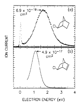
Figure 7.21. Yield of Cl- ions generated by attaching electrons of specified kinetic energy to saturated (a) and unsaturated cyclic hydrocarbon.
For the compound containing no olefinic group, the electron must attach directly to the C-Cl s* orbital (this process is endothermic by ca. 2 eV), whereas for the compound containing the vacant olefin p* orbital, the electron can attach (at ca. 1 eV) to this orbital. The result is that, for the unsaturated compound (b), the yield of Cl- ions is two orders of magnitude higher because capture into the p* orbital, followed by through-molecule electron transfer to the C-Cl bond is more efficient than direct capture into the C-Cl s* orbital followed by bond rupture. This example demonstrates a very important and widely applicable situation in which a functional group with a low-energy anti-bonding orbital serves as an antenna for low-energy electrons while a distant bond whose cleavage generates a radical of high electron affinity (e.g., the Cl radical here or the phosphate radical in the DNA example) is broken.
As a final example of electrons interacting with DNA fragments, we consider data from Professor Lars Andersen's group who uses a storage ring they call ELISA to effect collisions between electrons and, in this example, a base-sugar-phosphate unit. In Fig. 7.22, we see a depiction of the ELISA instrument showing its electrospray ion source.
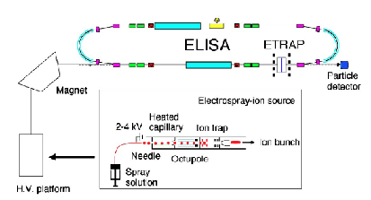
Figure 7.22. The Aarhus ELISA instrument.
In the experiments whose data we present here, the Andersen group used adenine- or uracil-containing fragments whose phosphate units were negatively charged. They then subjected these singly-charged anions to collisions with electrons of known kinetic energy and detected the abundances of neutral fragments that were produced subsequent to collion. In Fig. 7.23, we see plots of the cross-sections they inferred [[290]] for production of neutrals (they do not determine what neutrals) as functions of the anion-electron relative kinetic energy.
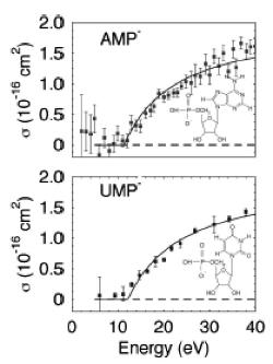
Figure 7.23. Plots of cross-sections for producing neutrals after collisions of AMP- or UMP- with electrons.
One of the main conclusions drawn from their analysis of this cross-section data is that it is consistent with a physical model in which energy is transferred through the Coulombic repulsion of the electron and the negatively charged phosphate group.
Professor Ron Naaman's group carries out experiments on electrons moving along DNA constitutent oligomers that are self-assembled and tied (usually with a thiol linkage) to a gold surface. In one experiment [[291]] whose set up is shown schematically in Fig. 7.24, they attach a double-strand DNA oligomer of known composition at one end to a gold electrode surface and at the other end to a gold nano-particle that serves as the other electrode. They hold the nano-particle on the end of an atomic force microscopy imaging tip. Finally, they apply a voltage V across the two electrodes and measure the current I that passes.
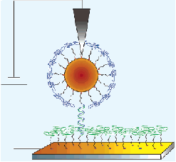
Figure 7.24. Schematic of single-strand DNA self-assembled and bound to a gold electrode surface (bottom) with a double-strand linker connected to a gold nano-particle serving as the other electrode.
In Fig. 7.25, we see the base composition of three double-strand oligomers used in ref. 291.
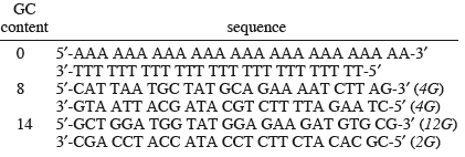
Figure 7.25. Base composition of three double-strand oligomers used in current-voltage experiments.
The current-voltage profiles obtained for these three oligomers are shown in Fig. 7.26. The inset in this figure shows the derivative dI/dV as a function of voltage for the oligomer containing no GC pairs.
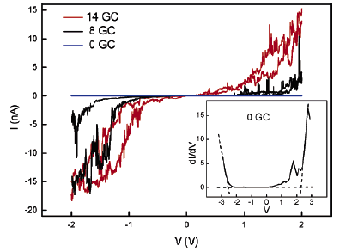
Figure 7.26. Current (I) obtained at a given applied voltage (V) for three double-strand oligomers.
The primary conclusion reached in ref. 291 is that the ability of double-stranded DNA to transport electrons along its chain is strongly dependent on the fraction of GC base pairs in the chain. As the fraction of GC pairs increases, so does the ability of the strand to allow current to flow.
Another result [[292]] from Professor Ron Naaman's lab sheds light on where counter cations can be located in DNA. I expect that most readers would expect these ions to be located near the negatively charged phosphate groups at least most of the time. However, there is considerable evidence that this is not the case. To illustrate, the Naaman group used a single-strand oligomer containing 14 A and 1 G bases to form self-assembled monolayers on a gold substrate. The 15-base oligomers, in a 0.4 M sodium phosphate buffer (pH = 7.2), were allowed to deposit onto the gold surface for various time durations. The gold surface with its attached oligomers was then rinsed in sodium phosphate buffer and rinsed three times for 20 min each time in deionized water and then stored in deionized water for 12 hr. After this, the surface was dried by a stream of N2 gas, after which X-ray photoelectron spectra (XPS) were taken. These spectroscopic measurements produced the data shown in Fig. 7.27.
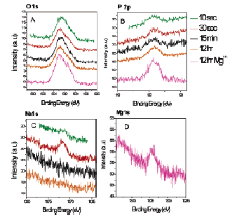
Figure 7.27. XPS spectra showing O, P, and Na intensities for oligomer solutions allowed to deposit from a sodium phosphate solution onto gold surface for 10 s, 30 s, 15 min, 12 hr. Also shown is the Mg intensity after 12 hr deposition from a magnesium phosphate solution.
By analyzing the XPS intensities, the authors of ref. 292 were able to determine the ratio of the numbers of nitrogen, carbon, oxygen, sodium, and phosphorous atoms as shown in Fig. 7.28.
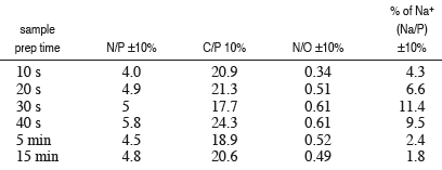
Figure 7.28. Atomic ratios for oligomer samples allowed to deposit for various time durations.
The C/P and N/P atomic ratios are reasonably independent of how long the oligomers were allowed to deposit onto the gold surface and are consistent with the 14A/1G composition of the sample. However, the Na/P ratio seems to increase with deposition time but to then fall off for times exceeding 30 s. In fact, in ref. 292 is was noted that, for a deposition time of several hours, no sodium is detected in the XPS spectra. If one Na+ cation were located near each negatively charged phosphate group, one would expect the Na/P ratio to be near unity. The speculation put forth in ref. 292 is that the Na+ ions are expelled and that protons enter to neutralize the phosphate groups as the samples are prepared and eventually dried by N2 gas.
Above we spoke about counter cations neutralizing the negative phosphate groups and we saw that, under some conditions, the counter ions may have even been replaced (e.g., by protons) as in the N2-dried oligomers used in ref. 292. Even when counter cations are present, it is known that both mono- and divalent cations (e.g., Na+, K+, Ca+2, and Mg+2) are not always spatially associated with the phosphate groups but can sometimes be found in DNA's grooves [[293]] near the bases. Under such conditions, one would expect the ability of DNA's bases to attract and bind an excess electron to be greatly altered (compared to conditions assumed in refs. 278 and 281). One would also expect that the rate at which base-attached electron can migrate to cleave a sugar-phosphate C-O bond would be greatly diminished in these conditions. So, it is very important to be aware of where,, at various times and under various conditions, the negative and postive charges reside within DNA.
One final example should serve to emphasize the importance of not assuming one knows where the negative and positive charges resides derives from work [[294]] that Professor Mathias Weber carried out in collaboration with other key groups in the area.
They carried out photoelectron spectroscopy experiments on single-strand oligonucleotides containing either five adenosine (A) or five thymidine (T) units connected by four phosphate groups. In both cases, the samples carried a negative charge of -4, each having lost a total of four protons. Although the primary focus of their study had been to measure effects due to the repulsive Coulomb barrier (we discussed this in Chapter 5), they observed spectral signatures that surprised them. In particular, at first, one might assume that in both of these samples, each of the four phosphate groups had lost a proton and hence was negatively charged. In this case, one would expect to see features in the photoelectron spectrum characteristic of detachment from a negative phosphate unit. However, the photoelectron specta were not consistent with these expectations. Specifically, the authors of ref. 294 concluded that at least one of the bases actually carried a negative charge. In other words, at least one of the bases had been deprotonated and at least one of the phosphate units was not negatively charged but instead had been protonated and was thus uncharged. In the author's opinion, it is likely that the four negative phosphate groups are, collectively, an extremely strong base that acts to abstract a proton from one of the DNA bases thus rendering it negatively charged.
IV. Electrons Fragmenting Peptides
All polypeptides and proteins consist of amino acids linked together by peptide bonds as shown in Fig. 7.29
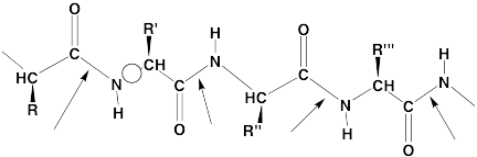
Figure 7.29. Representative sequence of peptide bonds (arrows) also showing the side chains (R through R''') and one of the N-Ca bonds (circle symbol) along a peptide backbone.
The amino acids' side chains can contain basic or acidic groups, so, depending on pH, they can be positively charged (e.g., as for a side chain containing an amine group that can be protonated at low pH) or negative (e.g., as for a side chain containing a carboxylic acid group that is deprotonated). In mass spectrometric probes of peptides' primary sequence (i.e., determining the order in which amino acids occur along the backbone), electrospray techniques are often used to transfer a sample from solution into the gas phase. If the solution is rendered acidic, some of the basic side chains are likely to be protonated, so the sample will be multiply positively charged when it enters the gas phase.
Two of the more powerful mass spectrometric tools for sequencing peptides makes use of electrons that attach to positively charged samples to cleave the peptide in a highly bond-selective manner. Specifically, it has been found that disulfide and N-Ca bonds in proteins and peptides are the most likely bonds to be ruptured when low-energy electrons attach to positively charged samples of these species in electron-capture dissociation [[295]] (ECD) or electron-transfer dissociation [[296]] (ETD) mass spectrometric experiments. However, why these bonds are preferentially cleaved and the mechanistic details of how this occurs are not fully understood.
The earliest proposed mechanism, suggested by two of the pioneers in the field, Professors Fred McLafferty and Roman Zubarev [[295]a] while at Cornell,

Fred McLafferty, Cornell

Roman Zubarev, Upsalla
posits that electron attachment occurs at a protonated site (that is probably hydrogen bonded to a nearby carbonyl or SS unit) to form a Rydberg (also called hypervalent) radical that subsequently transfers an H atom to the nearby carbonyl or SS unit to form a radical that can undergo facile S-S or N-Ca bond cleavage. This mechanism is described in Fig. 7.30 where the c/z notation used to describe the fragments produced by N-Ca cleavage is also illustrated.
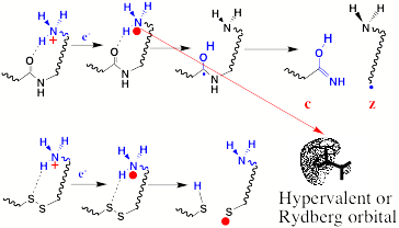
Figure 7.30. Cornell mechanism for N-Ca and S-S bond cleavage as electrons attach to positively charged peptides.
Notice that once the H atom transfers to the S-S bond, cleavage of this bond is immediate. However, after an H atom transfers to the carbonyl oxygen site to form the carbon-centered radical, a barrier must still be surmounted to break the N-Ca bond. However, this barrier is lowered by the fact that a C-N p bond is also formed as the N-Ca s bond breaks.
Although there was good precedent for the mechanism just discussed, certain experimental data prompted the author's group [[297]] to suggest that another mechanism may (also or instead) be operative. Our suggestion derived from evidence on S-S cleavage that was observed in disulfide-linked dimers of Ac-Cys-Alan-Lys (with n = 10, 15, and 20) protonated at the two terminal Lys sites shown in Fig. 7.31. Here, the alanine helices are shown in red, the cystine linkage containing the S-S bond appears in the center, and the two protonated Lys sites are at the left and right termini.
Figure 7.31. Structure of an (AcCA15K+H)22+ disulfide-linked dimer from [297] . The disulfide linkage is at the center and the two protonated sites are at the left and right ends.
Because very substantial S-S cleavage (and limited N-Ca cleavage near the termini) was observed under ECD conditions even when 20 alanines were present in each helix and even when the lysines were charged with Na+ cations rather than protons, we thought the Rydberg-based mechanism in Fig. 7.30 could not be operative in this case. How could the H atoms (or Na atoms) released from the lysine sites travel ca. 30 Å (when 20 alanines are present) to find the S-S bond?
We therefore examined [297] the possibility that the presence of positive charges (protons or Na+ ions) could Coulombically stabilize the S-S s* anti-bonding orbital rendering exothermic direct electron attachment to this s* orbital. In subsequent works, we [[298]] and Professor Frank Turecek's group [[299]] extended this suggestion to consider direct Coulomb-assisted attachment to amide p* orbitals to effect N-Ca backbone cleavages.

Frank Turecek, Washington
Professor Turecek has done as much as anyone to advance the theoretical understanding of peptide fragmentation in this and a number of other cases. The proposed mechanisms that we and the Turecek group put forth are described in Fig. 7.32.
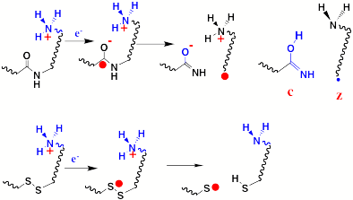
Figure 7.32. Coulomb-stabilized direct electron attachment to S-S s* or amide p* orbitals resulting in S-S or N-Ca bond cleavage.
In this mechanism, an electron first attaches to a Coulomb-stabilized S-S s* or amide p* orbital, then bond cleavage occurs, and finally neutralization of the negative site takes place.
To understand how the Coulomb-stabilized direct electron attachment works, let us consider the potential that acts on an excess electron in a peptide containing a positively charged protonated amine site such as shown in Fig. 7.33.
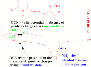
Figure 7.33. Potential experienced by an excess electron along peptide backbone near amide p* (left) and protonated amine (right) sites.
In the region of the protonated amine, the electron experiences a strong Coulombic attraction that can bind it by ca. 4 eV to form a Rydberg-attached state. What about near the amide site? We know from electron transmission spectroscopy experiments that attaching an electron to an amide p* orbital is endothermic by ca. 2.5 eV (to attach an electron to an S-S s* orbital is endothermic by ca. 1 eV). Thus, in the region of the amide p* orbital, while there exist attractive valence-range potentials acting on the electron, these potentials alone are not strong enough to render the p*-attached species electronically stable.
However, in a species containing both the amide p* orbital and one or more positively charged sites, the total potential experienced by an excess electron can be qualitatively different. In particular, the sum of the valence-range attractive potential of the p* orbital and the Coulomb potential can, as suggested in Fig. 7.33, produce a total potential in the region of the amide group that is strong enough to render the p*-attached species electronically stable. It is in this manner that we suggested the Coulomb potential facilitates direct attachment to amide p* or S-S s* orbitals.
Based on this Coulomb stabillizaton hypothesis, we considered model compounds containing either an S-S bond [[298]b] or an amide unit [[298]a] in addition to a protonated amine site at various distances (to vary the strength of the Coulomb stabilization) and we determined what happens when an electron attaches to the S-S s* or amide p* orbital. In Fig. 7.34, we show energy profiles appropriate to the S-S bond case in which the electron can bind either to the protonated site or to the S-S s* orbital.
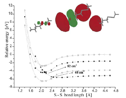
Figure 7.34. Energies of the parent +H3N-(CH3)3-SS-CH3 cation (open circles), ground Rydberg-attached (open squares), excited Rydberg (filled squares), and S-S s* attached (filled diamonds) species as functions of the S-S bond length.
The key things to glean from Fig. 7.34 are:
- It is ca. 4 eV exothermic to vertically (beginning near the equilibrium bond length of the parent cation) attach an electron to the ground-state Rydberg orbital (shown in Fig. 7.34 in the upper right).
- It is ca. 2 eV exothermic to vertically attach an electron to the excited Rydberg orbital (upper center in Fig. 7.34).
- It is also exotheric (by ca. 1.5 eV) to vertically attach an electron to the S-S s* orbital (upper left in Fig. 7.34).
- Once an electron attaches to the S-S s* orbital, the S-S bond promptly cleaves because this state's energy curve is repulsive.
It should be emphasized that the S-S s* curve, in the absence of the protonated amine site, would not lie below the curve of the parent cation; it is the presence of the positive site that, through its Coulomb potential, pulls the S-S s* state's curve down (by 14.4 eV/R, where R is the distance from the SS bond to the protonated amine). So, for compounds similar to that shown above but with varying distances between the S-S bond and the protonated site, this S-S s* curve will be shifted upward or downward in energy by various amounts of Coulomb stabilization.
When considering electron attachment to an amide p* orbital that has been Coulomb stabilized by one or more proximal positively charged groups, the story is similar but a bit more complicated because both the p* orbital to which the electron attaches and the N-Ca s* orbital to which an electron must be transferred play roles as illustrated in Fig. 7.35.
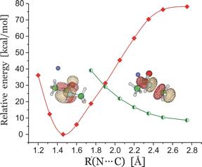
Figure 7.35. Energies of amide p*-attached (filled triangles) and N-Ca s*-attached (circles) states as functions of the N-Ca bond length. The curve corresponding to the species with no electron attached is not shown.
The primary difference between this case and the S-S bond cleavage case discussed earlier is that it is the Coulomb-stabilized amide p* orbital to which the electron initially attaches but, as the N-Ca bond elongates, the electron migrates into the Coulomb-stabilized N-Ca s* orbital thus cleaving this bond and forming a new C-N p bond in the process.
Another aspect of the electron attachment issue we had to address in our studies of ECD and ETD was whether an electron would prefer (i.e., have a larger cross-section or rate constant for) to attach to a positively charged site to form a Rydberg species or to an S-S s* or amide p* orbital that has been Coulomb stabilized. Energy considerations alone would suggest that attachment to the positively charged site should be favored because the binding energy at this site is large, but, as I now demonstrate, other factors come into play.
To address this issue, we used Landau-Zener theory [[298]c-e] to approximate the probabilities of an electron hopping from an anion (we used CH3- in our model studies) with a low electron binding energy (as used in ETD experiments) to a ground-state or excited-state Rydberg orbital or, alternatively, to a Coulomb-stabilized amide p* or SS s* orbital. To illustrate the ingredients that enter into such an evaluation, we show in Fig. 7.36 qualitative energy profiles for three pertinent electronic states as functions of the distance R between the H3C- anion and the positive site of the parent model cation H3C-(C=O)-(CH2)2-NH3+. These states pertain, respectively, to the following asymptotic situations:
- The H3C-(C=O)-(CH2)2-NH3+ cation and H3C- anion ion-pair state,
- The H3C-(C=O)-(CH2)2-NH3 Rydberg-state neutral and the H3C neutral radical,
- The H3C-(C=O)--(CH2)2-NH3+ p*-attached neutral and the H3C neutral radical.
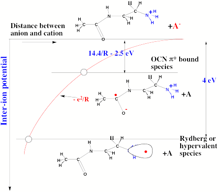
Figure 7.36. Qualitative energy profiles for ion-pair (steeply descending), Rydberg (lower flat), and amide p*-attached (upper flat) states as functions of the CH3- anion-amine distance.
In Landau-Zener (LZ) theory the probability P for an electron hopping from the H3C- anion to the model peptide during a collisional encounter is given by
![]() .
.
Here, H1,2 is the coupling matrix element that connects the ion-pair (H3C-(C=O)-(CH2)2-NH3+ + H3C-) state to either of the two electron transferred (H3C-(C=O)-(CH2)2-NH3 + H3C) states. These elements depend on the overlaps of the H3C- anion's carbon sp3 orbital from which the electron is transferred and the Rydberg or amide p* (or S-S s*) orbital into which it moves. DF is the difference in the slopes of the two energy surfaces at the point where the ion-pair and electron-transferred states cross, and v is the inter-ion speed at the point where this state-crossing occurs. By carrying out molecular dynamics collision simulations and evaluating all of the ingredients in the L-Z expression, we were able to compute the cross-sections for electron transfer from the ion-pair state to either the Rydberg or amide p* orbital
![]() ,
,
where RC is the distance at which the ion-pair and electron-transferred states cross.
From Fig. 7.36, we can see that:
- The RCvalue for transfer to the p* orbital is larger than for transfer to the Rydberg orbital; this larger RC favors transfer to the p* orbital in the cross-section.
- The slope difference DF and collision speeds v will be larger for the Rydberg-orbital transfer because the ions gain more kinetic energy in collisions that access the Rydberg's RC crossing. These factors will disfavor transfer to the Rydberg orbital, so, again transfer to the p* orbital is favored.
However, it turns out that the H1,2 matrix elements are considerably larger for connecting the H3C- orbital to the Rydberg orbital (ground or excited) than to the amide p* orbital. As a result, the cross-sections for transfer to the (ground or excited) Rydberg orbital turn out to be one to two orders of magnitude larger than for the amide p* (or S-S s*) orbital.
So, we concluded that the Cornell mechanism, which assumes electron capture at the positively charged site, could indeed be operative and even dominant if the S-S or amide group is close enough to the positive site to permit effective H-atom transfer. However, if the positive site is too far away for H-atom transfer, the Coulomb-stabilized S-S s* or amide p* attachment can provide the major contribution.
The suggestion that proximal positively charged groups can substantially alter the energy requirements and efficiencies of DEA processes can be of great significance to workers who study electron-induced bond fragmentation propensities in, for example, gas-phase mass spectrometric or ion-cyclotron resonance experiments on positively charged peptides and proteins. The research I detailed avove sheds light on how Coulomb stabilization can make direct attachment to low-energy anti-bonding orbitals (e.g., amide p* and SS s*) favorable and on to what extent electrons will attach to such orbitals (rather than to Rydberg orbitals of the positive sites).
References
[1] L. S. Cederbaum, Theor. Chim. Acta 31, 239 (1973).
[2] B. T. Pickup and O. Goscinski, Mol. Phys. 26, 1013 (1973); G. Purvis and Y. Öhrn, J. Chem. Phys. 60, 4063 (1975).
[3] For several examples, see the following papers: E. Clementi and A. D. McLean, Phys. Rev. A 133, 419 (1964); E. Clementi, A. D. McLean, D. L. Raimondi, and M. Yoshimine, Phys. Rev. A 133, 1274 (1964); E. Clementi, Phys. Rev. A 135, 980 (1964); A. C. Wahl and T. L. Gilbert, Bull Am. Phys. Soc., 10, 1097 (1965); W. T. Zemke, G. Das, and A. C. Wahl, Chem. Phys. Lett., 14, 310 (1972); P. E. Cade, J. Chem. Phys., 47, 2390 (1967); P. E. Cade, Proc. R. Soc., London Ser. A 91, 842 (1967); H. S. Taylor and F. E. Harris, J. Chem. Phys. 39, 1012 (1963); H. F. Schaefer and F. E. Harris, Phys. Rev. 170, 108 (1968); H. F. Schaefer and F. E. Harris, Phys. Rev. Lett. 21. 1561 (1968); E. R. Davidson, J. Chem. Phys. 36, 1080 (1962); D. Feller, L. E. McMurchie, W. T. Borden and E. R. Davidson, J. Chem. Phys. 77, 6134 (1982).
[4] J. C. Rienstra-Kiracofe, G. S. Tschumper, H. F. Schaefer, III, S. Nandi, and G. B. Ellison, Acc. Chem. Research, 102, 231 (2002).
[5] G. Herzberg, Molecular Spectra and Molecular Structure I. p. 512, Van Nostrand, New York (1950).
[6] A. Banerjee, R. Shepard, and J. Simons, Int. J. Quant. Chem: Quantum Chemistry Symposium 12, 389 (1978);
H. J. Monkhorst, Int. J. Quantum Chem. Symp. 11, 421 (1977); M. Nooijen and R. J. Bartlett, J. Chem. Phys. 102, 3629 (1995);
D. Mukhopadhyay, S. Mukhopadhyay, R. Chaudhuri, and D. Mukherjee, Theor. Chim. Acta 80, 441 (1991);
J. F. Stanton and R. J. Bartlett, J. Chem. Phys. 98, 7029 (1993);
R. J. Bartlett and J. F. Stanton, in Reviews in Computational Chemistry, edited by K. B. Lipkowitz and D. B. Boyd ~VCH, New York, 1994, Vol.5.
See, for example, J. V. Ortiz, Leszczynski, J. (Ed) Computational Chemistry: Reviews of Current Trends (Singapore: World Scientific) Vol 2 pp 1-61(1997)
[7] M. J. Frisch, G. W. Trucks, H. B. Schlegel, G. E. Scuseria, M. A. Robb, J. R. Cheeseman, J. A.Montgomery, Jr., T. Vreven, K. N. Kudin, J. C. Burant, J. M. Millam, S. S. Iyengar, J. Tomasi, V. Barone, B. Mennucci, M. Cossi, G. Scalmani, N. Rega, G. A. Petersson, H. Nakatsuji, M. Hada, M. Ehara, K. Toyota, R. Fukuda, J. Hasegawa, M. Ishida, T. Nakajima, Y. Honda, O. Kitao, H. Nakai, M. Klene, X. Li, J. E. Knox, H. P. Hratchian, J. B. Cross, C. Adamo, J. Jaramillo, R. Gomperts, R. E. Stratmann, O. Yazyev, A. J. Austin, R. Cammi, C. Pomelli, J. W. Ochterski, P. Y. Ayala, K. Morokuma, G. A. Voth, P. Salvador, J. J. Dannenberg, V. G. Zakrzewski, S. Dapprich, A. D. Daniels, M. C. Strain, O. Farkas, D. K. Malick, A. D. Rabuck, K. Raghavachari, J. B. Foresman, J. V. Ortiz, Q. Cui, A. G. Baboul, S. Clifford, J. Cioslowski, B. B. Stefanov, G. Liu, A. Liashenko, P. Piskorz, I. Komaromi, R. L. Martin, D. J. Fox, T. Keith, M. A. Al-Laham, C. Y. Peng, A. Nanayakkara, M. Challacombe, P. M.W. Gill, B. Johnson, W. Chen, M. W. Wong, C. Gonzalez, and J. A. Pople, Gaussian, Inc., Pittsburgh, PA, 2003.
[8] H. Hotop and W. C. Lineberger, J. Phys. Chem. Ref. Data 4, 539 (1975); J. Phys. Chem. Ref. Data 14, 731 (1985).
[9] T. Andersen, H. K. Haugen, and H. Hotop, J. Phys. Chem. Ref. Data 28, 1511 (1999).
[10] B. K. Janousk and J. I Brauman in Gas Phase Ion Chemistry; M. T. Bowers, Ed.; Academic Press, New York, 1979, Vol. 2.
[11] T. M. Miller, in CRC Handbook of Chemistry and Physics; R. C, West, M. J. Astle, and W. H. Beyer, Eds.; CRC Press; Boca Raton, FL, 1986; 66th ed.
[12] J. E. Bartmess, Negative Ion Energetics Data in NIST Chemistry Web-Book, NIST Standard Reference Database Number 69, W. G. Ballard and P. J. Linstrom, Eds.; National Institute of Standards and Technology: Gaithersburg, MD, February, 2000 (http://webbook.nist.gov).
[13] R. E. Continetti in Photoionization and Photodetachment; C. Y. Ng, Ed.; World Scientific, Inc: New York, 2000, Vol. II.
[14] J. C. Rienstra-Kiracofe, G. S. Tschumper, H. F. Schaefer, III, S. Nandi, and G. B. Ellison, Acc. Chem. Research, 102, 231 (2002).
[15] Nat. Stand. Ref. Data Ser. Nat. Bur. Stand. (U.S.) 26 (1969).
[16] As noted earlier, in refs. 8-14, what is presently known about atomic and molecular EAs can be found there.
[17] R. S. Berry,J. Chem. Phys. 45, 1228 (1966).
[18] J. Simons, J. Am. Chem. Soc. 103, 3971 (1981).
[19] A. Dreuw and L. S. Cederbaum, Phys. Rev. A 63, 012501 (2000)
[20] A.Dreuw and L. S. Cederbaum, Chem. Rev. 102, 181 (2002)
[21] A. I. Boldyrev, and J. Simons, J. Phys. Chem. 98, 2298 (1994);
A. Whitehead, R. Barrios, and J. Simons, J. Chem. Phys. 116, 2848 (2002)
[22] L-S Wang, C-F Ding, X-B Wang, and J. B. Nicholas, Phys. Rev. Lett. 81, 2667 (1998).
[23] See, for example, Qin Wu, Paul W. Ayers, and Weitao Yang, J. Chem. Phys. 119 2978 (2003).
[24] G. G. Schulz, Rev. Mod. Phys. 45, 378 (1973); 45, 423 (1973).
[25] K. D. Jordan and P. D. Burrow, Chem. Rev. 87, 557 (1987); A. Modelli, Trends in Chem. Phys. 6, 57 (1997).
[26] H. S. Carman, Jr., C. E. Klots, and R. N. Compton, in Isotope Effects in Gas-Phase Chemistry, edited by Jack A. Kaye, ACS Symposium Series 502 (American Chemical Society Press, 1992), p. 181.
[27] C. Desfrançois, Phys. Rev. A 51, 3667 (1995).
[28] D. M. Chipman, J. Chem. Phys. 118, 9937 (2003).
[29] T. M. Ramond, S. J. Blanksby, S. Kato, V. M. Bierbaum, G. E. Davico, R. L. Schwartz, W. C. Lineberger, and G. B, Ellison, J. Phys. Chem. A 106, 9641 (2002).
[30] S. J. Blanksby, T. M. Ramond, G. E. Davico, M. R. Nimlos, S. Kato, V. M. Bierbaum, W. C. Lineberger, G. B. Ellison, and M. Okumura, J. Am. Chem. Soc. 123, 9585 (2001).
[31] I. M. Waller, T. N. Kitsopoulos, and D. M. Neumark, J. Phys. Chem. 94, 2240 (1990).
[32] W.H. Robertson, E. G. Diken, E. A. Price, J-W Shin, and M. A. Johnson, Science, 299, 1367 (2003).
[33] L. Angel, M. K. Dogbevia, K. M. Rempala, and K. M. Ervin, J. Chem. Phys. 119, 8996 (2003).
[34] P. B. Armentrout, In The Encyclopedia of Mass Spectrometry. Volume 1: Theory and Ion Chemistry, Armentrout, P. B., Ed.; Elsevier: Amsterdam, 2003, 426-434.
[35] F. A. Akin and K. M. Ervin, J. Phys. Chem. A 110, 1342 (2006).
[36] R. R. Squires, V. M. Bierbaum, J. J. Grabowski, and C. H. DePuy, J. Am. Chem. Soc. 105, 5185 (1983).
[37] S. J. Blanksby, G. B. Ellison, V. M. Bierbaum, and S. Kato, J. Am. Chem. Soc, 124, 3196 (2002).
[38] A. T. Blades, Y. Ho, and P. Kebarle, J. Am. Chem. Soc. 118, 196 (1996).
[39] G. I. Gutsev and A. I. Boldyrev, Adv. Chem. Phys. 61, 169 (1985).
[40] J. Baker, R. H. Nobes, and L Radom, J. Comp. Chem. 7, 349 (1986).
[41] K. D. Jordan, Acc. Chem. Res. 12, 36 (1979)
[42] J. Simons and K. D. Jordan, Chem. Rev. 87, 535 (1987).
[43] J. Kalcher and A. F. Sax, Chem. Rev. 94, 2291 (1994); J. Kalcher, Ann. Reports, Sec. C, Royal Soc. of Chem. 93, 147-186 (1996).
[44] J. Kalcher, Ann. Reports, Sec. C, Royal Soc. of Chem. 93, 147 (1996).
[45] R. S. Berry, Chem. Rev. 69, 533 (1969).
[46] H. Massey, Negative Ions, Cambridge Univ. Press (1976), Cambridge, England.
[47] L. M. Branscomb, Atomic and Molecular Processes, edited by D. R. Bates, Academic Press, New York, N.Y. (1962).
[48] Recent Res. Devel. Phys. Chem., Theoretical Prospect of Negative Ions, J. Kalcher, ed., (2002).
[49] P. Nachtigall, K. D. Jordan, A. Smith and H. Jónsson, J.Chem.Phys. 104, 148 (1996).
[50] P. Skurski, M. Gutowski, and J. Simons, Int. J. Quantum Chem. 80, 1024 (2000).
[51] Professor Bob Parr, University of North Carolina.
http://net.chem.unc.edu/faculty/rgp/cfrgp01.html
He was among the first to push the density functional theory of Hohenberg and Kohn to bring it into the mainstream of electronic structure theory. For a good overview, see the book Parr R G and Yang W 1989 Density Functional Theory of Atoms and Molecules (New York, NY: Oxford Univ. Press)
[52] Professor Axel Becke, Queens University. He has been very actively involved in developing and improving exchange-correlation energy functionals.
For a good recent overview, see Becke A D 1995 Exchange-correlation approximations in density-functional theory in Yarkony D R (Ed) Modern Electronic Structure Theory (Singapore: World Scientific Publishing) Vol 2 pp 1022-1046; Becke A D Numerical Hartree-Fock-Slater calculations on diatomic molecules 1983 J.Chem.Phys. 76 6037-6045
[53] W. Kohn W and L. J. Sham, Phys.Rev. 140, A1133 (1965).
[54] For example, see Q. Wu, P. W. Ayers, and W. Yang, , J. Chem. Phys. 119, 2978 (2003); S. A. C. McDowell, R. D. Amos, and N. C. Handy, Chem. Phys. Lett. 235, 1 (1995)
[55] Many of the various density functional approaches that are under active development can be found in Jones R O 1987 Molecular calculations with the density functional formalism in Lawley K P (Ed) Advances in Chemical Physics (New York, NY: Wiley-Interscience) Vol LXVII pp 413-437; Dunlap B I Symmetry and degeneracy in Xa and density functional theory in Lawley K P (Ed) Advances in Chemical Physics (New York, NY: Wiley-Interscience) Vol LXIX pp 287-318; Dahl J P and Avery J (Eds) 1984 Local Density Approximations in Quantum Chemistry and Solid State Physics (New York, NY: Plenum); Parr R G Density functional theory, Ann.Rev.Phys.Chem. 34 631 (1983); D. R. Salahub, S. H. Lampson, and R. P. Messmer, Chem.Phys.Lett.85, 430 (1982); T. Ziegler, A. Rauk, and E. J. Baerends, Theor.Chim.Acta (Berl.) 43 261 (1977); A. D. Becke, J.Chem.Phys. 76, 6037 (1983); D. A. Case, Ann.Rev.Phys.Chem. 33, 151 (1982); J. K. Labanowski and J. W. Andzelm (Eds) 1991 Density Functional Methods in Chemistry (New York: Springer)
For a recent critical evaluation of situations where current DFT approaches experience difficulties, see E. R. Davidson, Inter. J. Quantum Chem. 69, 241 (1998).
[56] E. A. Hylleraas and B. Undheim, Z.Phys. 65, 759 (1930); J. K. L. MacDonald, Phys.Rev. 43, 830 (1933).
[57] J. A. Pople, Theoretical Models for Chemistry in Smith D W and McRae W B (Eds) Energy, Structure, and Reactivity (New York, NY: Wiley) p 51-67 (1983).
[58] B. O. Roos, P. R. Taylor and P. E. M. Siegbahn, Chem.Phys. 48 157 (1980).
[59] H. P. Kelly, Phys.Rev. 131, 684 (1963).
[60] Good early overviews of the electron propagator (that is used to obtain IP and EA data) and of the polarization propagator are given in P. Jørgensen and J. Simons, 1981 Second Quantization Based Methods in Quantum Chemistry (New York, NY: Academic Press)
The very early efforts on these methods are introduced in Linderberg J and Öhrn Y 1973 Propagator Methods in Quantum Chemistry (New York, NY: Academic Press)
More recent summaries include: L. S. Cederbaum and W Domcke, Adv.Chem.Phys. 36, 205 (1977); J. Oddershede, Adv.Chem.Phys. 69, 201 (1987); J. V. Ortiz, 1997 The Electron Propagator Picture of Molecular Electronic Structure in Leszczynski J (Ed) Computational Chemistry: Reviews of Current Trends (Singapore: World Scientific) Vol 2 pp 1-61
[61]The introduction of equations of motion (EOM) for energy differences and for operators that connect two states appears first in the nuclear physics literature; see for example, D. J. Rowe, Rev.Mod.Phys. 40 153 (1968).
I applied these ideas to excitation energies in atoms and molecules in 1971; see Eqs. (2.1-2.6) in J. Simons, J.Chem.Phys. 55 1218 (1971).
In a subsequent treatment from the time-dependent response point of view, connection with the Greens function methods was made: J. Simons, J.Chem.Phys. 57 3787 (1972).
In 1973, the EOM method was then extended to treat IP and EA cases: J. Simons, J.Chem.Phys. 58 4899 (1973).
A more recent overview of much of the EOM, Greens function, and propagator field is given in J. Oddershede, Adv.Chem.Phys. 69 201 (1987)
[62] J. Simons, J.Chem.Phys. 58 4899 (1973). A recent overview of the history of this author's efforts and of how the EOM methods have evolved can be accessed in Equations of Motion (EOM) Methods for Computing Electron Affinities, "Encyclopedia of Computational Chemistry", J. Simons, (2004).
[63] J. Olsen and P. Jørgensen, 1995 Time-dependent response theory with applications to self-consistent field and multiconfigurational self-consistent field wave functions in Yarkony D R (Ed) Modern Electronic Structure Theory (Singapore: World Scientific Publishing) Vol 2 pp 857-990
[64]A good overview of the recent status is given in Bartlett R J 1995 Coupled-cluster theory an overview of recent developments in Yarkony D R (Ed) Modern Electronic Structure Theory (Singapore: World Scientific Publishing) Vol 2 pp 1047
[65] D. Feller, J. Chem. Phys. 96, 6104 (1992); 98, 7059 (1993).
A. Halkier, T. Helgaker, P. Jørgensen, W. Klopper and J. Olsen, Chem. Phys. Lett. 302, 437 (1999).
[66] C. Schwartz, Phys. Rev. 126, 1015 (1962); Meth. Comp. Phys. 2, 241(1963).
Valeev, E. F.; Allen, W. D.; Hernandez, R.; Sherrill, C. D.; Schaefer, H. F. J. Chem. Phys.118, 8594 (2003).
[67] Strategies for locating transition states are detailed in, for example, J. A. Nichols, H. Taylor, P. P. Schmidt, and J. Simons, J. Chem. Phys. 92, 340 (1990).
[68] P. Jørgensen, and J. Simons, eds., Geometrical Derivatives of Energy Surfaces and Molecular Properties, D. Reidel Publishing Company (1985); T. Helgaker, P. Jørgensen, and J. Olsen, Molecular Electronic Structure Theory, John Wiley and Sons (2000).
[69] K. D. Jordan, Acc. Chem. Res. 12, 36 (1979).
[70] J. Kalcher, Ann. Reports, Sec. C, Royal Soc. of Chem. 93, 147 (1996).
[71] P. K. Acharya, R. A. Kendall and J. Simons, SASP 84 (1984); P. K. Acharya, R. A. Kendall and J. Simons, J. Am. Chem. Soc. 106, 3402 (1984); P. K. Acharya, R. A. Kendall and J. Simons, J. Chem. Phys. 83, 3888 (1985); G. Chalasinski, R. A. Kendall, H. Taylor, and J. Simons, J. Phys. Chem. 92, 3086 (1988); D. O'Neal and J. Simons, J. Phys. Chem. 93, 58 (1988); J. Simons, J. Chem. Phys. 91, 6858 (1989); J. Simons, J. Am. Chem. Soc. 103, 3971 (1981).
[72] K. R. Lykke, D. M. Neumark, T. Andersen, V. J. Trapa, and W. C. Lineberger, J. Chem. Phys. 87, 6842 (1987).
D. M. Neumark, K. R. Lykke, T. Andersen and W. C. Lineberger, J. Chem. Phys. 83, 4364 (1985).
T. Andersen, K. R. Lykke, D. M. Neumark and W. C. Lineberger, J. Chem. Phys. 86, 1858 (1987).
J. Marks, D. M. Wentzel, P. B. Comita, and J. I. Brauman, J. Chem. Phys. 86, 5284 (1986).
F. K. Meyer, J. M. Jasinski, R. N. Rosenfeld and J. I. Brauman, J. Am. Chem. Soc. 104, 663 (1982).
R. N. Rosenfeld, J. M. Jasinski and J.I. Brauman,J. Chem. Phys. 71, 1030 (1979);
R. D. Mead, K. R. Lykke, W. C.Lineberger, J. Marks and J. I. Brauman, J. Chem. Phys. 81, 4883 (1984).
R. L. Jackson, A. H. Zimmerman and J. I. Brauman,J. Chem. Phys.71, 2088 (1979).
A. H. Zimmerman, K. J. Reed and J. I. Brauman, J. Am. Chem. Soc. 99, 7203 (1977).
A. H. Zimmerman and J. I. Brauman,J. Chem. Phys. 66, 5823 (1977);
C. A. Wight, and J. L. Beauchamp, J. Am. Chem. Soc. 103, 6501 (1981).
[73] F. K. Meyer, J. M. Jasinski, R. N. Rosenfeld, and J. I. Brauman, J. Am. Chem. Soc. 104, 663 (1982).
[74] C. A. Wight and J. L. Beauchamp, J. Phys. Chem. 88, 4426 (1984).
[75] H. M. Lee, S. B. Suh, and K. S. Kim, J. Chem. Phys. 119, 7685 (2003).
[76] T. B. Arthur, M. Peschke, P. Kebarle, Int. J. Mass Spec. 228, 1017 (2003).
[77] J. Smets, W. J. McCarthy, and L. Adamowicz, J. Phys. Chem. 100, 14655 (1996).
[78] S. Carles, C. Desfrançois, J. P. Schermann, D. M. A. Smith and L. Adamowicz, J. Chem. Phys. 112, 3726 (2000).
[79] C. Desfrançois, Phys. Rev. A 51, 3667 (1995).
[80] E. Fermi, E. Teller, Phys. Rev.72, 399 (1947).
[81] A.S. Wightman, Phys. Rev., 77, 521 (1950).
[82] P. Serra and S. Kais, Chem. Phys. Lett. 372, 205 (2003).
[83] F. Wang and K. D. Jordan, Ann. Rev. Phys. Chem. 54, 367 (2003).
[84] M. Gutowski, K. D. Jordan, and P. Skurski, J Phys. Chem. 102, 2624 (1998).
[85] O.H. Crawford, Proc. Roy. Soc. (London) 91, 279 (1967).
[86] O.H. Crawford and A. Dalgarno, Chem. Phys. Lett. 1, 23 (1967).
[87] W.B. Brown and R.E. Roberts, J. Chem. Phys. 46, 2006 (1967).
[88] J. E. Turner, Am. J. Physics, 45, 758 (1977).
[89] O. H. Crawford and W. R. Garrett, J. Chem. Phys. 66, 4968 (1977).
[90] F. Wang and K. D. Jordan, J. Chem. Phys. 116, 6961 (2002); F. Wang and K. D. Jordan, J. Chem. Phys. 114, 10717 (2001).
[91] M. Gutowski, P. Skurski, A. I. Boldyrev, J. Simons, and K. D. Jordan, Phys. Rev. 54, 1906 (1996).
[92] H. Abdoul-Carime and C. Desfrançois, Eur. Phys. J. D 2, 149 (1998).
[93] K.D. Jordan, W. Luken, J. Chem. Phys., 1976, 64, 2760; see also, K. D. Jordan, Acc. Chem. Res. 12, 36 (1979).
[94] K. D. Jordan, Acc. Chem. Res. 12, 36 (1979); M. Gutowski and P. Skurski, Recent Res. Dev. Phys. Chem. 3, 245 (1999); J. Simons and P. Skurski, A Theoretical Prospect of Negative Ions in Recent Res. Devel. Phys. Chemistry, Research Signpost, Trivandrum (2001); F. Wang and K. D. Jordan, Ann. Rev. Phys. Chem. 54, 367 (2003).
[95] K. D. Jordan, K. M. Griffing, J. Kenney, E. L. Andersen and J. Simons, J. Chem. Phys. 64, 4730 (1976).
[96] K.D. Jordan and J.J. Wendoloski, Chem. Phys. 21, 145 (1977).
[97] Y. Yoshioka and K.D. Jordan, J. Chem. Phys. 73, 5899 (1980).
[98] M. Gutowski, P. Skurski, A.I. Boldyrev, J. Simons, K.D. Jordan, Phys. Rev. A 54, 1906 (1996).
[99] M. Gutowski, P. Skurski, J. Simons, and K.D. Jordan, Int. J. Quantum Chem. 64, 183 (1997).
[100] L. Adamowicz and E.A. McCullough, Chem. Phys. Lett. 107, 72 (1984).
[101] L. Adamowicz and E.A. McCullough, Jr., J. Phys. Chem. 88, 2045 (1984).
[102] L. Adamowicz and R.J. Bartlett, Jr., J. Chem. Phys. 83, 6268 (1985).
[103] L. Adamowicz and R.J. Bartlett Chem. Phys. Lett. 129, 159 (1986).
[104] L. Adamowicz and R.J. Bartlett, J. Chem. Phys. 88, 313 (1988).
[105] L. Adamowicz, J. Chem. Phys. 91, 7787 (1989).
[106] G.L. Gutsev and L. Adamowicz, Chem. Phys. Lett. 246, 245 (1995).
[107] N.A. Oyler and L. Adamowicz, J. Phys. Chem. 97, 11122 (1993).
[108] N.A. Oyler and L. Adamowicz, Chem. Phys. Lett. 219, 223 (1994).
[109] G.H. Roehrig, N.A. Oyler, and L. Adamowicz, Chem. Phys. Lett. 225, 265 (1994).
[110] G.H. Roehrig, N.A. Oyler, and L. Adamowicz, J. Phys. Chem. 99, 14285 (1995).
[111] G.L. Gutsev, A.L. Sobolewski, and L. Adamowicz, Chem. Phys. 196, 1 (1995).
[112] J. Smets, W.J. McCarthy, and L. Adamowicz, J. Phys. Chem. 100, 14655 (1996).
[113] J. Smets, W.J. McCarthy, and L. Adamowicz, Chem. Phys. Lett. 256, 360 (1996).
[114] J. Smets, D.M.A. Smith, Y. Elkadi, and L. Adamowicz, J. Phys. Chem. A 101, 9152 (1997).
[115] J. Smets, D.M.A. Smith, Y. Elkadi, and L. Adamowicz, Pol. J. Chem. 72, 1615 (1998).
[116] D.M.A. Smith, J. Smets, Y. Elkadi, and L. Adamowicz, J. Phys. Chem. A 101, 8123 (1997).
[117] Y. Elkadi and L. Adamowicz, Chem. Phys. Lett. 261, 507 (1996).
[118] D.M. Chipman, J. Phys. Chem. 83, 1657 (1979).
[119] G.L. Gutsev, M. Nooijen, and R.J. Bartlett, Chem. Phys. Lett. 267, 13 (1997).
[120] G.L. Gutsev, M. Nooijen, and R.J. Bartlett, Phys. Rev. A 57, 1646 (1998).
[121] G.L. Gutsev and R.J. Bartlett, J. Chem. Phys. 105, 8785 (1996).
[122] M. Gutowski and P. Skurski, J. Chem. Phys. 107, 2968 (1997).
[123] M. Gutowski and P. Skurski, J. Phys. Chem. B 101, 9143 (1997).
[124] P. Skurski and M. Gutowski, J. Chem. Phys. 108, 6303 (1998).
[125] M. Gutowski and P. Skurski, Chem. Phys. Lett. 300, 331 (1999).
[126] P. Skurski and M. Gutowski, J. Chem. Phys. 111, 3004 (1999).
[127] M. Gutowski, P. Skurski, and J. Simons, J. Am. Chem. Soc.122, 10159 (2000).
[128] R. Barrios, P. Skurski, J. Rak, and M. Gutowski, J. Chem. Phys. 113, 8961 (2000).
[129] P. Skurski, M. Gutowski, and J. Simons, J. Chem. Phys. 114, 7443 (2001).
[130] J. Rak, P. Skurski, and M. Gutowski, J. Chem. Phys.114, 10673 (2001).
[131] Y. Boutellier, C. Desfrançois, H. Abdoul-Carime, and J.P. Schermann, J. Chem. Phys. 105, 6420 (1996).
[132] H. Abdoul-Carime and C. Desfrançois, Eur. Phys. J. D 2, 149 (1998).
[133] P. Skurski, M. Gutowski, and J. Simons, J. Chem. Phys. 110, 274-280 (1999).
[134] P. Skurski, M. Gutowski, and J. Simons, J. Phys. Chem. A 103, 625 (1999.
[135] A.H. Zimmerman and J.I. Brauman, J. Chem. Phys. 66, 5823 (1977).
[136] R.L. Jackson, A.H. Zimmerman, and J.I. Brauman, J. Chem. Phys. 71, 2088 (1979).
[137] R.L. Jackson, P.C. Hiberty, and J.I. Brauman, J. Chem. Phys. 74, 3705 (1981).
[138] J. Marks, P.B. Comita, and J.I. Brauman, J. Am. Chem. Soc. 107, 3718 (1985).
[139] J. Marks, D.M. Wetzel, P.B. Comita, and J.I. Brauman, J. Chem. Phys. 84, 5284 (1986).
[140] D.M. Wetzel and J.I. Brauman, J. Chem. Phys. 90, 68 (1989).
[141] E.A. Brinkman, S. Berger, J. Marks, and J.I. Brauman, J. Chem. Phys. 99, 7586 (1993).
[142] B.C. Romer and J.I. Brauman, J. Am. Chem. Soc. 119, 2054 (1997).
[143] R.D. Mead, K.R. Lykke, W.C. Lineberger, J. Marks, and J.I. Brauman, J. Chem. Phys. 81, 4883 (1984).
[144] T. Andersen, K.R. Lykke, D.M. Neumark, and W.C. Lineberger, J. Chem. Phys. 86, 1858 (1987).
[145] K.R. Lykke, D.M. Newmark, T. Andersen, V.J. Trapa, and W.C. Lineberger, J. Chem. Phys. 87, 6842(1987).
[146] J. Marks, J.I. Brauman, R.D. Mead, K.R. Lykke, and W.C. Lineberger, J. Chem. Phys. 88, 6785 (1988).
[147] A.S. Mullin, K.K. Murray, C.P. Schultz, D.M. Szaflarski, and W.C. Lineberger, Chem. Phys. 166, 207 (1992).
[148] A.S. Mullin, K.K. Murray, C.P. Schultz, and W.C. Lineberger, J. Phys. Chem. 97, 10281 (1993).
[149] K. Yokoyama, G.W. Leach, J.B. Kim, and W.C. Lineberger, J. Chem. Phys. 105, 10696 (1996).
[150] K. Yokoyama, G.W. Leach, J.B. Kim, W.C. Lineberger, A.I. Boldyrev, and M. Gutowski, J. Chem. Phys. 105, 10706 (1996).
[151] C. Desfrançois, N. Khelifa, A. Lisfi, J.P. Schermann, J.G. Eaton, and K.H. Bowen, J. Chem. Phys. 95, 7760 (1991).
[152] C. Desfrançois, B. Baillon, J.P. Schermann, S.T. Arnold, J.H. Hendricks, and K.H. Bowen, Phys. Rev. Lett. 72, 48 (1994).
[153] C. Desfrançois, H. Abdoul-Carime, C. Adjouri, N. Khelifa, and J.P. Schermann, Europhys. Lett. 26, 25 (1994).
[154] C. Desfrançois, H. Abdoul-Carime, N. Khelifa, J.P. Schermann, V. Brenner, and P. Millie, J. Chem. Phys. 102, 4952 (1995).
[155] C. Desfrançois, H. Abdoul-Carime, C.P. Schulz, and J.P. Schermann, Science269, 1707 (1995).
[156] C. Desfrançois, Phys. Rev. A 51, 3667 (1995).
[157] C. Desfrançois, H. Abdoul-Carime, and J.P. Schermann, J. Chem. Phys. 104, 7792 (1996).
[158] R.N. Compton, H.S. Carman, Jr., C. Desfrançois, H. Abdoul-Carime, J.P. Schermann, J.H. Hendricks, S.A. Lyapustina, and K.H. Bowen, J. Chem. Phys. 105, 3472 (1996).
[159] C. Desfrançois, H. Abdoul-Carime, and J.P. Schermann, Int. J. Mod. Phys. B 10, 1339 (1996).
[160] H. Abdoul-Carime, A. Wakisaka, Y. Bouteiller, C. Desfrançois, and J.P. Schermann, Z. Phys. D 40, 55 (1997).
[161] H. Abdoul-Carime, W. Wakisaka, J. Flugge, H. Takeo, V. Periquet, J.P. Schermann, and C. Desfrançois, J. Chem. Soc. Faraday Trans. 93, 4289 (1997).
[162] C. Desfrançois, V. Periquet, Y. Boutellier, and J.P. Schermann, J. Phys. Chem. A 102, 1274 (1998).
[163] C. Desfrançois, V. Periquet, C. Carles, J.P. Schermann, and L. Adamowicz, Chem. Phys. 239, 475 (1998).
[164] C.E.H. Dessent, C.G. Bailey, and M.A. Johnson, J. Chem. Phys. 103, 2006 (1995).
[165] J.A.D. Stockdale, F.J. Davis, R.N. Compton, and C.E. Klots, J. Chem. Phys. 60, 4279 (1974).
[166] R.N. Compton, P.W. Reinhardt, and C.D. Cooper, J. Chem. Phys., 68, 4360 (1978).
[167] J.V. Coe, G.H. Lee, J.G. Eaton, S.T. Arnold, H.W. Sarkas, and K.H. Bowen, Jr., J. Chem. Phys. 92, 3980 (1990).
[168] J. H. Hendricks, H.L. de Clercq, S.A. Lyapustina, C.A. Fancher, T.P. Lippa, J.M. Collins, S.T. Arnold, G.H. Lee, and K.H. Bowen, in Proceedings of the Yamada Conference No. XLIII, May 1995, Structure and Dynamics of Clusters, Universal Academy Press: Tokyo, 1995.
[169] J. H. Hendricks, S.A. Lyapustina, H.L. de Clercq, J.T. Snodgrass, and K.H. Bowen, Jr., J. Chem. Phys. 104, 7788 (1996).
[170] A.W. Castelman, Jr., and K.H. Bowen, Jr., J. Phys. Chem. 100, 12911 (1996).
[171] J.H. Hendricks, H.L. de Clercq, S.A. Lyapustina, and K.H. Bowen, Jr., J. Chem. Phys. 107, 2962 (1997).
[172] C.E.H. Dessent, C.G. Bailey, and M.A. Johnson, J. Chem. Phys. 103, 2006 (1995).
[173] C.E.H. Dessent, J. Kim, and M.A. Johnson J. Phys. Chem. 100, 12 (1996).
[174] D. Serxner, C.E.H. Dessent, and M.A. Johnson, J. Chem. Phys. 105, 7231 (1996).
[175] C.E.H. Dessent, J. Kim, and M.A. Johnson, Acc. Chem. Res. 31, 527 (1998).
[176] C.G. Bailey, C.E.H. Dessent, M.A. Johnson, and K.H. Bowen, Jr., J. Chem. Phys. 104, 6976 (1996).
[177] P. D. Burrow, G. A. Gallup, A. M. Scheer, S. Denifl, S. Ptasinska, T. Märk, and P. Scheier, J. Chem. Phys. 124, 124310 (2006).
[178] This molecule also has a valence-bound anion in addition to the dipole-bound state we refer to here.
[179] P. Skurski, M. Gutowski, and J. Simons, Int. J. Quantum Chem. 80, 1024 (2000).
[180] F. Wang and K. D. Jordan, J. Chem. Phys. 114, 10717 (2001).
[181] O. H. Crawford and W. R. Garrett, J. Chem. Phys. 66, 4968 (1977). In this paper, the authors examine a rotating FFD model and determine how large m must be to effect electron binding for various rotational constants (i.e., various moments of inertia).
[182] K. R. Lykke, D. M. Neumark, T. Andersen, V. J. Trapa, and W. C. Lineberger, J. Chem. Phys. 87, 6843 (1987).
[183] J.V. Coe, G.H. Lee, J.G. Eaton, S.T. Arnold, H.W. Sarkas, and K.H. Bowen, Jr., J. Chem. Phys. 92, 3980 (1990);
[184] R. D. Mead, K. R. Lykke, W. C. Lineberger, J. Marks, and J. I. Brauman, J. Chem. Phys. 81, 4883 (1984).
[185] D. C. Clary, J. Phys. Chem. 92, 3173 (1988).
[186] L. D. Landau and E. M. Lifschitz, Quantum Mechanics (2nd Ed.), Pergamon Press, Oxford, England (1965).
[187] This trial function was suggested by Professor E. R. Davidson in August of 1998 in a personal communication to J. S. We are most appreciative for the thougtful analysis given to this problem by Professor Davidson.
[188] K. D. Jordan and J. F. Liebman, Chem. Phys. Lett. 62, 143 (1979).
[189] M. Gutowski and P. Skurski, Chem. Phys. Lett. 303, 65 (1999).
[190] R. N. Compton, F. B. Dunning, and P. Nordlander, Chem. Phys. Lett. 253, 8 (1996).
[191] C. Desfrançois, Y. Bouteiller, and J. P. Schermann, D. Radisic, S.T. Stokes, and K. H. Bowen, N. I. Hammer and R. N. Compton, Phys. Rev. Letters 92, 27 (2004).
[192] C. Desfrançois, V. Periquet, S. A. Lyapustina, T. P. Lippa, W. Robinson, K. H. Bowen, H. Nonaka, and R. N. Compton, J. Chem. Phys. 111, 4569 (1999).
[193] I. Anusiewicz, P. Skurski, and J. Simons, J. Phys. Chem. A, 106, 10636 (2003).
[194] C. Desfrançois, Y. Bouteiller, J. P. Scherman, D. Radisic, S.T. Stokes, K.H. Bowen, N.I. Hammer, R.N. Compton. Phys. Rev. Lett. 92, 083003 (2004).
[195] H. Abdoul-Carime and C. Defrancois, Eur. Phys. J. D2, 149 (1998); C. Defrancois, H. Abdoul-Carime, N. Khelifa, and J. P. Schermann, J. Chim. Phys. 92, 409 (1995).
[196] P. Skurski, J. Rak, and J. Simons, J. Chem. Phys., 115, 11193 (2001).
[197] R. N. Compton, A. A. Tuinman, C. E. Klots, Mark R. Pederson, and David C. Patton, Phys. Rev. Letters, 78 4367 (1997).
[198] S. Difley and J. Simons, Inter. J. Quantum Chem. 105, 507 (2006).
[199] See, for example, G. Herzberg, Faraday Discuss. Chem. Soc. 71, 165 (1981) and G.I. Gellene, D.A. Cleary, and R. Porter, J. Chem. Phys. 77, 3471 (1982).
[200] K.H. Bowen and J.G. Eaton, The Structure of Small Molecules and Ions, R. Naaman and Z. Vager, Eds., Plenum Press: New York, 1987, p 147
[201] J.V. Ortiz, J. Chem. Phys. 87, 3557-3562 (1987); M. Gutowski, H. Taylor, R. Hernandez and J. Simons, J. Phys. Chem. 92, 6179 (1988); J. Simons and M. Gutowski, Chem. Rev. 91, 669 (1991).
[202] J. Kalcher, P. Rosmus, and M. Quack, Can. J. Phys. 62, 1323 (1983).
[203] M. Gutowski, and J. Simons, J. Chem. Phys., 93, 3874 (1990).
[204] M. Gutowski, H. Taylor, R. Hernandez, and J. Simons, J. Phys. Chem. 92, 6179 (1988).
[205] P. Skurski, M. Gutowski, R. Barrios, and J. Simons, Chem. Phys. Lett. 337, 143 (2001); P. Skurski, and J. Simons, J. Chem. Phys. 115, 8373 (2001).
[206] P. Skurski, J. Rak, J. Simons, and M. Gutowski, J. Am. Chem. Soc. 123, 11073 (2001)
[207] A. Sawicka, P. Skurski, and J. Simons, Chem. Phys. Lett. 362, 572 (2002).
[208] P. Skurski, M. Gutowski and J. Simons, Int. J. Quant. Chem., 76, 197 (2000).
[209] C. Sarasola, J. E. Fowler, and J. M. Ugalde, J. Chem. Phys. 110, 11717 (1999); C. Sarasola, J. E. Fowler, J., M. Elorza, and J. M. Ugalde, Chem. Phys. Lett. 337, 355 (2001).
[210] P. Skurski and J. Simons, J. Chem. Phys, 112, 6563 (2000).
[211] L.-S. Wang and X-B. Wang, J. Phys. Chem. 104, 1978 (2000).
[212] J. Simons, P. Skurski, and R. Barrios, J. Am. Chem. Soc. 122, 11893 (2000).
[213] P. Skurski, M. Gutowski, and J. Simons, Chem. Phys. Lett. 322, 175 (2000).
[214] T. Sommerfeld, J. Phys. Chem., A104, 8806 (2000)
[215] M. Gutowski, A. I. Boldyrev, J. V. Ortiz, and J. Simons, J. Am. Chem. Soc., 116, 9262-9268 (1994).
[216] P. Weis, O. Hampe, S. Gilb, and M. M. Kappes, Chem. Phys. Lett. 321, 426 (2000).
[217] A. I. Boldyrev and J. Simons, J. Chem. Phys. 97, 2826 (1992).
[218] M. K. Scheller, R. N. Compton, and L. S. Cederbaum, Science, 270 1160-1166 (1995).
[219] H-G. Weikert, L. S. Cederbaum, F. Tarantelli, and A. I. Boldyrev, Z. Phys. D 18, 229 (1991); H-G. Weikert and L. S. Cederbaum, J. Chem. Phys. 99, 8877 (1993).
[220] A. Dreuw and L. S. Cederbaum, Chem. Rev., 102, 181 (2002)
[221] A. I. Boldyrev, and J. Simons, J. Chem. Phys., 97, 2826 (1992)
[222] L-S Wang and X-B Wang, J. Phys. Chem. A 104, 1978 (2000).
[223] J. Jackowski and J. Simons, J. Am. Chem. Soc., 125, 16089 (2003).
[224] J. Novoa, P. Lafuente, R. E. Del Sesto, and J. S. Miller, Angew. Chem. Int. Ed., 40, 2540 (2001).
[225] A. U. Hazi and H. S. Taylor, Phys. Rev. A1, 1109 (1970). Also, see S. Feuerbacher, T. Sommerfeld, and L. S. Cederbaum, J. Chem. Phys. 121, 6628 (2004) as well as B. Nestmann and S. D. Peyerimhoff, J. Phys. B 18, 615 (1985).
[226] J. Simons, J. Chem. Phys. 75, 2465 (1981); R. F. Frey and J. Simons, J. Chem. Phys. 84, 4462 (1986).
[227] S. Feuerbach, T. Sommerfeld and L. S. Cederbaum, J. Chem. Phys. 121, 6628 (2004); S. Feuerbacher, T. Sommerfeld and L. S. Cederbaum, J. Chem. Phys. 121, 6624 (2004).
[228] S. Feuerbacher and L. S. Cederbaum, J. Phys. Chem. A 109, 11401 (2005); S. Feuerbacher and L. S. Cederbaum, J. Chem. Phys. 124, 044320 (2006).
[229] K. Ervin, I. Anusiewicz, P. Skurski, J. Simons, and W. C. Lineberger, J. Phys. Chem. A 107, 8521 (2003).
[230] M. Mucha, T. Frigato, L. M. Levering, H. C. Allen, D. J. Tobias, L. X. Dang, and P. Jungwirth, J. Phys. Chem. B 109, 7617 (2005).
[231] E. A. Price, N. I. Hammer, and M. A. Johnson, J. Phys. Chem. A 108, 3910 (2004).
[232] E. M. Myshakin, W. H. Robertson, G. H. Weddle, K, D. Jordan, and M. A. Johnson, J. Chem. Phys. 118, 4945 (2003).
[233] A. Sanov and W. C. Linebeger, Phys. Chem. Chem. Phys. 6, 2018 (2004).
[234] S.E. Bradforth, P. Jungwirth, Phys. Chem., 106, 1286 (2002).
[235] A. Banerjee, R. Shepard, and J. Simons, J. Chem. Phys. 73, 1814-1826 (1980).
[236] J.V. Coe, G. H. Lee, J. G. Eaton, S. T. Arnold, H. W. Sarkas, K. H. Bowen, C. Ludewigt, H. Haberland, and D. R. Worsnop, J. Chem. Phys. 92. 3960 (1990).
[237] R. N. Barnett, U. Landman, C. L. Cleveland, and J. Jortner, J. Chem. Phys. 88, 4429 (1988).
[238] J. V. Coe, Int. Rev. in Phys. Chem. 20, 33 (2001).
[239] J. R. R. Verlet, A. E. Bragg, A. Kammrath, O. Cheshnovsky, and D. M. Neumark, Science 307, 93 (2005); A. E. Bragg, J. R. R. Verlet, A. Kammrath, O. Cheshnovsky, and D. M. Neumark, Science 306, 669 (2004).
[240] J. Kim, L. Becker, O. Cheshnovsky, and M. A. Johnson, Chem. Phys. Lett. 297, 90 (1998).
[241] D. H. Paik, I-R. Lee, D-S. Yang, J. S. Baskin, and A. H. Zewail, Science, 306, 672 (2004)
[242] A nice overview is given in K. D. Jordan, Science, 306, 618 (2004).
[243] L. Turi, W-S. Sheu, and P. J. Rossky, Science 309, 914 (2005).
[244] G. Makov and A. Nitzan, J. Phys. Chem. 98, 3459 (1994).
[245] T. Sommerfeld and K. D. Jordan, J. Am. Chem. Soc., 128, 5828 (2006).
[246] N. I. Hammer, J-W. Shin, J. M. Headrick, E. G. Diken, J. R. Roscioli, G. H. Weddle, and M. A. Johnson, Science 306, 675 (2004).
[247] H. M. Lee, S. Lee, and K. S. Kim, J. Chem. Phys. 119, 187 (2003).
[248] J. M. Herbert and M. Head-Gordon, J. Am. Chem. Soc. 128, 13932 (2006).
[249] P. Skurski, and J. Simons, J. Chem. Phys. 115, 10731 (2001).
[250] P. Skurski, and J. Simons, J. Chem. Phys. 116, 6118 (2002).
[251] M.-K. Tsai, F. Wang, and K. D. Jordan, J. Phys. Chem. A 108 2912 (2004).
[252] D. M. Neumark, Acc. Chem. Res. 26, 33 (1993); D. M. Neumark, J. Chem. Phys. 125, 132303 (2006).
[253] R. L. Schwartz, G. E. Davico, J. B. Kim, and W. C. Lineberger, J. Chem. Phys. 112, 4966 (2000).
[254] H. Hopper, M. Lococo, O. Dolgounitcheva, V. G. Zakrzewski, and J. V. Ortiz, J. Am. Chem. Soc., 122, 12813 (2000).
[255] I. Anusiewicz, P. Skurski, and J. Simons, J. Phys. Chem. A 106, 10634 (2002).
[256] K.H. Bowen and J.G. Eaton, The Structure of Small Molecules and Ions, R. Naaman and Z. Vager, Eds., Plenum Press: New York, 1987, p 147
[257] J.V. Ortiz, J. Chem. Phys. 87, 3557-3562 (1987); M. Gutowski, H. Taylor, R. Hernandez and J. Simons, J. Phys. Chem. 92, 6179 (1988); J. Simons and M. Gutowski, Chem. Rev. 91, 669 (1991).
[258] M. L. Kimble, A. W. Castleman, R. Mitric, C. Burgel, V. Bonacic-Koutecky, J. Am. Chem. Soc., 126, 2526 (2004)
[259] B.D. Leskiw, A. W. Castleman, C. Ashman, S.N. Khanna, J. Chem. Phys., 2001, vol. 114, iss. 3, pp 1165
[260] B. C. Guo 1, K. P. Kerns, and A. W. Castleman Jr., Science 255, 1411 (1992); B. C. Guo, S. Wei, J. Purnell, S. A. Buzza, and A. W. Castleman, Jr. Science 256, 515 (1992).
[261] See ref. 260 as well as A. I. Boldyrev and J. Simons, J. Am. Chem. Soc. 119, 4618 (1997).
[262] L-S. Wang, S, Li, and H. Wu, J. Phys. Chem. 100, 19211 (1996).
[263] J. Ho, K. M. Ervin, and W. C. Lineberger, J. Chem. Phys. 93, 6987 (1990).
[264] O. C. Thomas, W. Zheng, S. Xu, and K. H. Bowen, Jr. Phys. Rev. Lett. 89, 213403-1 (2002).
[265] A. I. Boldyrev and J. Simons, J. Am. Chem. Soc. 120, 7967 (1998).
[266] X. Li, L-S. Wang, A. I. Boldyrev, and J. Simons, J. Am. Chem. Soc, 121, 6033 (1999).
[267] A. I. Boldyrev and L-S. Wang, Chem. Rev. 105, 3716 (2005).
[268] S. Carles, C. Desfrançois, J. P. Schermann, D. M. A. Smith and L. Adamowicz, J. Chem. Phys. 112, 3726 (2000).
[269] N. A. Richardson, S. S. Wesolowski, and H. F. Schaefer, III, J. Am. Chem. Soc., 107, 848 (2003).
[270] N. A. Richardson, S. S. Wesolowski, and H. F. Schaefer, III, J. Phys. Chem. B 124, 10163 (2002).
[271] M. Sobczyk and J. Simons, Inter. J. Mass. Spec. 253, 274 (2006).
[272] J. Simons, Acc. Chem. Res. 39, 772 (2006).
[273] K. Aflatooni, G. A. Gallup, and P. D. Burrow, J. Phys. Chem. A 102, 6205 (1998).
[274] M. Allan, J. Phys. B., At. Mol. Opt. Phys. 39, 2939 (2006).
[275] S. Tonzani and C. H. Greene, J. Chem. Phys. 124, 1 (2006).
[276] C. Desfrançois, V. Periquet, Y. Bouteiller, and J. P. Schermann, J. Phys. Chem. A 102, 1274 (1998).
[277] P. D. Burrow, G. A. Gallup, A. M. Scheer, S. Denifl, S. Ptasinska, T. Märk, and P. Scheier, J. Chem. Phys. 124, 124310 (2006).
[278] B. Boudaiffa, P. Cloutier, D. Hunting, M. A. Huels, and L. Sanche, Science, 287, 1658 (2000).
[279] S. Ptasinska, S. Denifl, V. Grill, T. D. Märk, P. Scheier, S. Gohlke, M. A. Huels, and E. Illenberger, Angew. Chem. Int. Ed. 44, 1647 (2005).
[280] H. Abdoul-Carime, S. Gohlke, E. Fischbach, J. Scheinke, and E. Illenberger, Chem. Phys. Lett. 387, 267 (2004).
[281] R. Barrios, P. Skurski, and J. Simons, J. Phys. Chem. B 106, 7991 (2002)
[282] Attachment of low-energy electrons to DNA bases has been studied using electron transmission spectroscopy in K. Aflatooni, G. A. Gallup, and P. D. Burrow, J Phys. Chem. A 102, 6205 (1998).
[283] Among all the components of DNA, including its water solvent, it is the p orbitals of the bases that produce the lowest-energy unoccupied molecular orbitals (LUMOs), the p* orbitals.
[284] J. Berdys, I. Anusiewicz, P. Skurski, and J. Simons, J. Am Chem. Soc. 126, 6441 (2004)
[285] J. Berdys, P. Skurski, and J. Simons, J. Phys. Chem. B 108, 5800 (2004).
[286] I. Anusiewicz , J. Berdys, M. Sobczyk, P. Skurski, and J. Simons, J. Phys. Chem. A 108, 11381 (2004).
[287] F. Martin, P. D. Burrow, Z. Cai, P. Cloutier, D. Hunting, and L. Sanche,
Phys. Rev. Lett. 93, 068101-1 (2004); Y. Zheng, P. Cloutier, D. Hunting, L. Sanche, and J. R. Wagner, J. Am. Chem. Soc. 127, 16592 (2005); Y. Zheng, P. Cloutier, D. Hunting, R. Wagner, and L. Sanche, J. Chem. Phys. 124, 064710-1 (2006).
[288] J. Gu,Y. Xie, and H. F. Schaefer, III, J. Am. Chem. Soc. 128, 1250 (2006).
[289] D. M. Pearl, P. D. Burrow, J. J. Nash, H. Morrison, and K. D. Jordan, J. Am. Chem. Soc., 115, 9876 (1993).
[290] H. Bluhme, M. J. Jensen, S. Brøndsted Nielsen, U. V. Pedersen, K. Seiersen, A. Svendsen, and L. H. Andersen, Phys. Rev. A 70, 020701 (2004).
[291] C. Nogues, S. R. Cohen, S. Daube, N. Apter, and R. Naaman, J. Phys. Chem. B 110, 8910 (2006).
[292] S. G. Ray, H. Cohen, R. Naaman, and Y. Rabin, J. Am. Chem. Soc. 127, 17138 (2005).
[293] a. F. C. Marincola, V. P. Denisov, and B. Halle, J. Am. Chem. Soc. 126, 6739-6750 (2004);
- S. G. Ray, H. Cohen, R. Naaman, and Y. Rabin J. Am. Chem. Soc.,127, 17138 (2005);
- E. Clementi and G. Corongiu, Biomolecular Stereodynamics, Vol. I, R.H. Sarma Ed., Adenine Press, N.Y., pp. 209-260, (1981);
- E. Clementi and G. Corongiu, Biopolymers 21, 763 (1982).
[294] J. M. Weber, I. N. Ioffe, K. M. Berndt, D. Löffler, J. Friedrich, O. T. Ehrler, A. S. Danell, J. H. Parks, and M. M. Kappes, J. Am. Chem. Soc, 126, 8585 (2004).
[295] a. R. A. Zubarev, N. L. Kelleher, and F. W. McLafferty, J. Am. Chem. Soc., 120, 3265 (1998).
- R. A. Zubarev, N. A. Kruger, E. K. Fridriksson, M. A. Lewis, D. M. Horn, B. K. Carpenter, and F. W. McLafferty, J. Am. Chem. Soc. 121, 2857 (1999).
- R. A. Zubarev, D. M. Horn, E. K. Fridriksson, N. L. Kelleher,N. A. Kruger, M. A. Lewis, B. K. Carpenter, and F. W. McLafferty, Anal. Chem. 72, 563 (2000).
- R. A. Zubarev, K. F. Haselmann, B. Budnik, F. Kjeldsen, and F. Jensen, Eur. J. Mass Spectrom, 8, 337 (2002).
[296] a. J. E. P. Syka, J. J. Coon, M. J. Schroeder, J. Shabanowitz, and D. F. Hunt, Proc. Nat. Acad. Sci., 101, 9528 (2004).
- J. J. Coon, J. E. P. Syka, J. C. Schwartz, J. Shabanowitz, and D. F. Hunt, Inter. J. Mass Spec., 236, 33 (2004).
- S. J.Pitteri, P. A. Chrisman, and S. A.McLuckey, Anal. Chem., 77, 5662 (2005).
- H. P. Gunawardena, M. He, P. A. Chrisman, S. J. Pitteri, J. M.Hogan, B. D. M. Hodges, and S. A. McLuckey, J. Am. Chem. Soc., 127, 12627 (2005).
[297] A. Sawicka, P. Skurski, R. R. Hudgins, and J. Simons, J. Phys. Chem. B107, 13505 (2003).
[298] a. I. Anusiewicz , J. Berdys, M. Sobczyk, A. Sawicka, P. Skurski, and J. Simons, J. Phys. Chem. A109, 250 (2005);
- A. Sawicka, J. Berdys-Kochaska, P. Skurski, and J. Simons, Inter. J. Quantum Chem. 102 838 (2005);
- I. Anusiewicz, J. Berdys-Kochanska, and J. Simons, J. Phys. Chem. A109, 5801 (2005);
- I. Anusiewicz, J. Berdys-Kochanska, P. Skurski, and J. Simons, J. Phys. Chem. A 110, 1261 (2006);
- M. Sobczyk and J. Simons, J. Phys. Chem. B 110, 7519 (2006);
- M. Sobczyk and J. Simons, Inter. J. Mass. Spec., 253 274 (2006).
[299] E. A. Syrstad, and F., J. Turecek, J. Am. Soc. Mass Specrom.,16, 208 (2004).